SSD Object Detection
SSD Object Detection
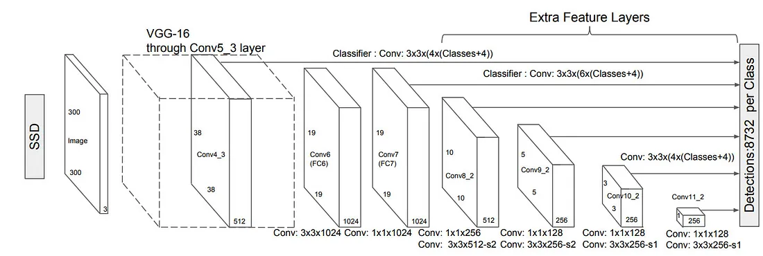
Layers
- In SSD OD we have multiple layers, each layer has
m x npoints on the feature map. Each point corresponds topanchor boxes. Therefore at each layer we havem x n x pnumber of priors. - Each anchor should represent an object therefore for each prior we have
Cclasses and4regression values for a box. - Therefore for each featuremap the output channel depth of the conv layers for classification is
p x Cand for regression inp x 4(pmight be different for each featuremap)
Sample Backbone
	self.model = nn.Sequential(
            conv_bn(3, self.base_channel, 2),  # 160*120
            conv_dw(self.base_channel, self.base_channel * 2, 1),
            conv_dw(self.base_channel * 2, self.base_channel * 2, 2),  # 80*60
            conv_dw(self.base_channel * 2, self.base_channel * 2, 1),
            conv_dw(self.base_channel * 2, self.base_channel * 4, 2),  # 40*30
            conv_dw(self.base_channel * 4, self.base_channel * 4, 1),
            conv_dw(self.base_channel * 4, self.base_channel * 4, 1),
            conv_dw(self.base_channel * 4, self.base_channel * 4, 1),
            conv_dw(self.base_channel * 4, self.base_channel * 8, 2),  # 20*15
            conv_dw(self.base_channel * 8, self.base_channel * 8, 1),
            conv_dw(self.base_channel * 8, self.base_channel * 8, 1),
            conv_dw(self.base_channel * 8, self.base_channel * 16, 2),  # 10*8
            conv_dw(self.base_channel * 16, self.base_channel * 16, 1)
        )

	regression_headers = ModuleList([
        SeperableConv2d(in_channels=base_net.base_channel * 4, out_channels=p * 4, kernel_size=3, padding=1),
        SeperableConv2d(in_channels=base_net.base_channel * 8, out_channels=p * 4, kernel_size=3, padding=1),
        SeperableConv2d(in_channels=base_net.base_channel * 16, out_channels=p * 4, kernel_size=3, padding=1),
        Conv2d(in_channels=base_net.base_channel * 16, out_channels=p * 4, kernel_size=3, padding=1)
    ])

    classification_headers = ModuleList([
        SeperableConv2d(in_channels=base_net.base_channel * 4, out_channels=p * num_classes, kernel_size=3, padding=1),
        SeperableConv2d(in_channels=base_net.base_channel * 8, out_channels=p * num_classes, kernel_size=3, padding=1),
        SeperableConv2d(in_channels=base_net.base_channel * 16, out_channels=p * num_classes, kernel_size=3, padding=1),
        Conv2d(in_channels=base_net.base_channel * 16, out_channels=p * num_classes, kernel_size=3, padding=1)
    ])
How Priors are Formed:
Depending to the number of layers we form the priors. The lower layers are associated to smaller bounding boxes and the deeper layers to bigger bounding boxes.
We normalize all the prior boxes with respect to the image size. The center of each prior box is between each feature map pixel (i + .5, j + .5).
The formula to create scales for SSD anchors is based on a linear interpolation between a minimum and a maximum scale. The scales are distributed evenly across the number of feature maps used by the SSD model. The formula is as follows:
s_k = s_{min} + \frac{s_{max} - s_{min}}{m - 1}\times (k - 1)
where
- where $s_k$ is the $k^{th}$ feature map.
- $s_{min}$ is the minimum scale (typically a small value, such as 0.1).
- $s_{max}$ is the maximum scale (typically a larger value, such as 0.9).
- $m$ is the total number of feature maps.
- $k$ is the index of the feature map, ranging from 1 to $m$.
Code to generate the scales
def generate_scales(s_min, s_max, num_feature_maps):
    """
    Generate scales for SSD anchors using linear interpolation.

    Args:
        s_min (float): Minimum scale (e.g., 0.1).
        s_max (float): Maximum scale (e.g., 0.9).
        num_feature_maps (int): Number of feature maps.

    Returns:
        scales (list): A list of scales for each feature map.
    """
    scales = [s_min + (s_max - s_min) * k / (num_feature_maps - 1) for k in range(num_feature_maps)]
    return scales

# Example usage
s_min = 0.1
s_max = 0.9
num_feature_maps = 6

scales = generate_scales(s_min, s_max, num_feature_maps)
print("Generated scales:", scales)
Explanation:
- $s_{min}$: The minimum scale value.
- $s_{max}$: The maximum scale value.
- num_feature_maps: The number of feature maps for which you want to generate scales.
- The generate_scales function uses a linear interpolation to generate scales evenly between $s_{min}$ and $s_{max}$.
This code will generate scales for the anchor boxes that are evenly distributed between the minimum and maximum scale values, suitable for use in SSD.
Scales are created then we create priors. Like this
import numpy as np

def generate_ssd_anchors(feature_map_sizes, aspect_ratios, scales):
    """
    Generate anchor boxes for SSD.

    Args:
        feature_map_sizes (list of tuples): Sizes of the feature maps, e.g., [(38, 38), (19, 19), ...].
        aspect_ratios (list of lists): Aspect ratios for each feature map.
        scales (list of floats): Scales for each feature map.

    Returns:
        anchors (list): A list of anchor boxes in the form [cx, cy, width, height].
    """
    anchors = []

    for idx, (feature_map_size, scale) in enumerate(zip(feature_map_sizes, scales)):
        fm_height, fm_width = feature_map_size
        for i in range(fm_height):
            for j in range(fm_width):
                # Center of the anchor box
                cx = (j + 0.5) / fm_width
                cy = (i + 0.5) / fm_height

                # Generate anchor boxes for each aspect ratio
                for ratio in aspect_ratios[idx]:
                    width = scale * np.sqrt(ratio)
                    height = scale / np.sqrt(ratio)
                    anchors.append([cx, cy, width, height])

                    # Add an anchor with the square aspect ratio (s')
                    if ratio == 1.0:
                        scale_next = np.sqrt(scale * scales[min(idx + 1, len(scales) - 1)])
                        anchors.append([cx, cy, scale_next, scale_next])

    return np.array(anchors)

# Example usage
feature_map_sizes = [(38, 38), (19, 19), (10, 10), (5, 5), (3, 3), (1, 1)]
aspect_ratios = [[1, 2, 0.5], [1, 2, 3, 0.5, 1/3], [1, 2, 3, 0.5, 1/3], [1, 2, 3, 0.5, 1/3], [1, 2, 0.5], [1, 2, 0.5]]
scales = [0.1, 0.2, 0.375, 0.55, 0.725, 0.9]

anchors = generate_ssd_anchors(feature_map_sizes, aspect_ratios, scales)
print("Generated anchors shape:", anchors.shape)
It is important to note that the output of the ssd is two tensors:
- Conf: batch_size x num_priors x num_classes
- Prediction: batch_size x num_priors x 4
Therefore, we have to create similar input ground truth as well:
- Labels = batch_size x num_priors
- Location = batch_size x num_priors x 4
For this in the transform we create assign_prior function to convert the ground truth to the output desired.
To match ground truth bounding boxes with SSD anchor boxes and calculate the Intersection over Union (IoU), we follow a series of steps:
-
Convert Bounding Boxes Format: Ground truth bounding boxes are typically given in the $[x_{min}, y_{min}, x_{max}, y_{max}]$ format, while SSD anchor boxes are usually in the $[c_x, c_y, w, h]$ format. We first need to convert these formats for comparison.
-
Calculate IoU: Intersection over Union (IoU) is a metric used to measure the overlap between two bounding boxes. It is defined as the area of the intersection divided by the area of the union of the two bounding boxes.
Steps to Convert Bounding Boxes and Calculate IoU
- Convert anchor boxes from $[c_x, c_y, w, h]$ to $[x_{min}, y_{min}, x_{max}, y_{max}]$.
- Compute the intersection area between each anchor box and the ground truth bounding box.
- Calculate the union area.
- Compute the IoU.
Code to Convert Bounding Boxes and Calculate IoU
Here’s how to implement this:
import numpy as np

def convert_to_corners(cx, cy, w, h):
    """
    Convert center-format bounding boxes to corner-format.

    Args:
        cx, cy: Center x and y coordinates.
        w, h: Width and height of the box.

    Returns:
        x_min, y_min, x_max, y_max: Corner coordinates of the box.
    """
    x_min = cx - w / 2
    y_min = cy - h / 2
    x_max = cx + w / 2
    y_max = cy + h / 2
    return x_min, y_min, x_max, y_max

def calculate_iou(box1, box2):
    """
    Calculate the Intersection over Union (IoU) of two bounding boxes.

    Args:
        box1: [x_min, y_min, x_max, y_max] for the first box.
        box2: [x_min, y_min, x_max, y_max] for the second box.

    Returns:
        IoU: Intersection over Union score.
    """
    # Calculate intersection coordinates
    x_min_inter = max(box1[0], box2[0])
    y_min_inter = max(box1[1], box2[1])
    x_max_inter = min(box1[2], box2[2])
    y_max_inter = min(box1[3], box2[3])

    # Compute intersection area
    inter_width = max(0, x_max_inter - x_min_inter)
    inter_height = max(0, y_max_inter - y_min_inter)
    intersection_area = inter_width * inter_height

    # Compute areas of the two boxes
    area_box1 = (box1[2] - box1[0]) * (box1[3] - box1[1])
    area_box2 = (box2[2] - box2[0]) * (box2[3] - box2[1])

    # Compute union area
    union_area = area_box1 + area_box2 - intersection_area

    # Calculate IoU
    iou = intersection_area / union_area if union_area > 0 else 0
    return iou

# Example usage
# Ground truth box: [x_min, y_min, x_max, y_max]
ground_truth_box = [0.3, 0.3, 0.7, 0.7]

# Anchor box in [cx, cy, w, h] format
anchor_box = [0.5, 0.5, 0.4, 0.4]

# Convert anchor box to corner format
anchor_box_corners = convert_to_corners(*anchor_box)

# Calculate IoU
iou = calculate_iou(ground_truth_box, anchor_box_corners)
print("IoU:", iou)
Explanation
-
convert_to_corners: This function converts anchor boxes from the center format $[c_x, c_y, w, h]$ to the corner format $[x_{min}, y_{min}, x_{max}, y_{max}]$ to make IoU calculation easier.
-
calculate_iou: This function calculates the IoU between two bounding boxes using the intersection and union areas.
Matching Ground Truth with Anchors
To match ground truth bounding boxes with anchor boxes in SSD:
- Calculate the IoU for each anchor box with each ground truth box.
- Assign each ground truth box to the anchor box with the highest IoU.
- Use a threshold (e.g., 0.5) to determine whether an anchor box is a positive or negative match. This process helps the SSD model learn to predict accurate bounding boxes and object classes.
Assigning ground truth labels and bounding boxes to priors (or anchor boxes) is a crucial step in training an SSD model. The process involves matching each ground truth bounding box with the best-suited anchor boxes (priors) and assigning labels accordingly. Here’s a detailed explanation of how this is typically done:
Steps to Assign Ground Truth Labels and Bounding Boxes to Priors:
- Compute IoU for Each Prior with Each Ground Truth Box
- Calculate the Intersection over Union (IoU) between each prior and all ground truth boxes. The IoU measures the overlap between two bounding boxes and is used to determine how well a prior matches a ground truth box.
- Assign Each Ground Truth Box to the Best-Matching Prior
- For each ground truth box, find the prior with the highest IoU and assign the ground truth box to this prior. This ensures that each ground truth box is matched with at least one prior.
- Set the corresponding label of the best-matching prior to the class of the ground truth box and update the bounding box coordinates.
- Assign Remaining Priors Based on IoU Threshold
- For priors that have not been assigned a ground truth box, assign a ground truth box if the IoU exceeds a certain threshold (e.g., 0.5). This step ensures that priors with sufficient overlap with any ground truth box are also used for training.
- If a prior does not meet the threshold, it is assigned as background (negative sample).
Code to Assign Ground Truth Labels and Bounding Boxes to Priors Here is a PyTorch implementation of the process:
import torch

def assign_ground_truth(priors, ground_truth_boxes, ground_truth_labels, iou_threshold=0.5):
    """
    Assign ground truth boxes and labels to priors (anchor boxes).

    Args:
        priors: Tensor of shape [num_priors, 4], each row is [cx, cy, w, h] for priors.
        ground_truth_boxes: Tensor of shape [num_objects, 4], each row is [xmin, ymin, xmax, ymax] for ground truth.
        ground_truth_labels: Tensor of shape [num_objects], containing class labels for each ground truth box.
        iou_threshold: Float, IoU threshold to consider a prior as a positive match.

    Returns:
        loc_targets: Tensor of shape [num_priors, 4], containing the assigned bounding box coordinates.
        labels: Tensor of shape [num_priors], containing the assigned class labels.
    """
    num_priors = priors.size(0)
    num_objects = ground_truth_boxes.size(0)

    # Initialize labels and loc_targets
    labels = torch.zeros(num_priors, dtype=torch.long)  # Background class (0) for all priors initially
    loc_targets = torch.zeros(num_priors, 4, dtype=torch.float32)  # Placeholder for bounding box coordinates

    # Compute IoU between each prior and each ground truth box
    iou = compute_iou(priors, ground_truth_boxes)  # Shape: [num_priors, num_objects]

    # Step 1: Match each ground truth box to the best prior
    best_prior_iou, best_prior_idx = iou.max(dim=0)  # Best prior for each ground truth box
    best_truth_iou, best_truth_idx = iou.max(dim=1)  # Best ground truth for each prior

    # Ensure that each ground truth box is assigned to at least one prior
    best_truth_idx[best_prior_idx] = torch.arange(num_objects)
    best_truth_iou[best_prior_idx] = 1.0

    # Step 2: Assign labels and bounding boxes to priors
    pos_mask = best_truth_iou > iou_threshold  # Positive mask for priors with IoU above the threshold
    labels[pos_mask] = ground_truth_labels[best_truth_idx[pos_mask]]  # Assign class labels
    assigned_boxes = ground_truth_boxes[best_truth_idx[pos_mask]]  # Get the assigned ground truth boxes

    # Convert ground truth boxes to [cx, cy, w, h] format
    cxcywh_boxes = convert_to_cxcywh(assigned_boxes)
    loc_targets[pos_mask] = cxcywh_boxes  # Assign bounding box coordinates

    return loc_targets, labels

def compute_iou(priors, boxes):
    """
    Compute the Intersection over Union (IoU) between priors and ground truth boxes.

    Args:
        priors: Tensor of shape [num_priors, 4], each row is [cx, cy, w, h] for priors.
        boxes: Tensor of shape [num_objects, 4], each row is [xmin, ymin, xmax, ymax] for ground truth.

    Returns:
        iou: Tensor of shape [num_priors, num_objects], containing IoU values.
    """
    # Convert priors to corner format [xmin, ymin, xmax, ymax]
    priors_corners = convert_to_corners(priors)

    # Compute intersection and union areas
    intersection = compute_intersection(priors_corners, boxes)
    area_priors = (priors_corners[:, 2] - priors_corners[:, 0]) * (priors_corners[:, 3] - priors_corners[:, 1])
    area_boxes = (boxes[:, 2] - boxes[:, 0]) * (boxes[:, 3] - boxes[:, 1])
    union = area_priors.unsqueeze(1) + area_boxes.unsqueeze(0) - intersection

    return intersection / union  # Return IoU values
Helper functions to convert bounding boxes to different formats would be implemented here
Helper functions to convert bounding boxes to different formats would be implemented here Explanation Initialization:
- labels: A tensor initialized to 0 (background class) for all priors. loc_targets: A tensor initialized to zero for storing the bounding box coordinates.
IoU Calculation:
-
compute_iou: A helper function that calculates the IoU between each prior and each ground truth box. Matching Ground Truth to Priors: Best Prior for Each Ground Truth Box: Ensures that every ground truth box is matched with at least one prior. Positive Matches: Priors with an IoU greater than iou_threshold are considered positive matches.
-
Assigning Labels and Bounding Boxes: Positive Mask: Used to update the labels and bounding box coordinates for positive matches. Background Priors: Priors that do not meet the IoU threshold remain assigned to the background class. This process ensures that the SSD model has positive and negative examples to learn from, with properly assigned labels and bounding boxes.
MultiBox Loss Function
The MultiBox Loss function used in SSD (Single Shot MultiBox Detector) is a combination of two losses: localization loss and confidence loss.
- Localization Loss: This is a regression loss (Smooth L1 Loss) used to measure how well the predicted bounding box matches the ground truth.
- Confidence Loss: This is a classification loss (Cross-Entropy Loss) that measures how well the model classifies each anchor as an object or background.
Below is a PyTorch implementation of the MultiBox Loss function for SSD:
import torch
import torch.nn as nn

class MultiBoxLoss(nn.Module):
    def __init__(self, num_classes, overlap_threshold=0.5, neg_pos_ratio=3):
        super(MultiBoxLoss, self).__init__()
        self.num_classes = num_classes
        self.overlap_threshold = overlap_threshold
        self.neg_pos_ratio = neg_pos_ratio
        self.loc_loss = nn.SmoothL1Loss(reduction='none')  # No reduction to keep per-element loss
        self.conf_loss = nn.CrossEntropyLoss(reduction='none')  # No reduction for per-element loss

    def forward(self, predictions, targets):
        loc_preds, conf_preds = predictions  # loc_preds: [batch_size, num_anchors, 4], conf_preds: [batch_size, num_anchors, num_classes]
        loc_targets, conf_targets = targets  # loc_targets: [batch_size, num_anchors, 4], conf_targets: [batch_size, num_anchors]

        # Compute localization loss
        pos_mask = conf_targets > 0  # Mask for positive anchors; shape: [batch_size, num_anchors]
        loc_loss = self.loc_loss(loc_preds[pos_mask], loc_targets[pos_mask])  # Compute loss only for positive anchors
        loc_loss = loc_loss.mean()  # Mean localization loss across all positive samples
        # Compute confidence loss
        # Flatten the predictions and targets for easier computation of CrossEntropyLoss
        conf_loss = self.conf_loss(
            conf_preds.view(-1, self.num_classes),  # Flattened class predictions: [batch_size * num_anchors, num_classes]
            conf_targets.view(-1)  # Flattened class targets: [batch_size * num_anchors]
        )
        # Reshape back to [batch_size, num_anchors] for hard negative mining
        conf_loss = conf_loss.view(conf_preds.size(0), -1)  # Shape: [batch_size, num_anchors]

        # Split the confidence loss into positive and negative losses
        pos_loss = conf_loss[pos_mask]  # Confidence loss for positive anchors; shape: [num_positive_samples]
        neg_loss = conf_loss[~pos_mask]  # Confidence loss for negative anchors; shape: [num_negative_samples]

        # Hard negative mining: Select top-k negative samples
        num_pos = pos_mask.sum(dim=1, keepdim=True)  # Number of positive anchors per batch; shape: [batch_size, 1]
        num_neg = torch.clamp(self.neg_pos_ratio * num_pos, max=neg_loss.size(1))  # Number of negative samples per batch; shape: [batch_size, 1]

        # Sort negative losses in descending order and select the top-k
        neg_loss, _ = neg_loss.sort(dim=1, descending=True)  # Sort negative losses; shape: [batch_size, num_negative_samples]
        neg_loss = neg_loss[:, :num_neg.squeeze()]  # Select top-k negative losses; shape: [batch_size, num_neg]

        # Combine positive and negative losses and calculate the mean
        conf_loss = torch.cat([pos_loss, neg_loss], dim=1)  # Combined loss; shape: [batch_size, num_pos + num_neg]
        conf_loss = conf_loss.mean()  # Mean confidence loss across the batch

        # Total loss
        total_loss = loc_loss + conf_loss  # Sum of localization and confidence loss
        return total_loss
Explanation
- Inputs:
- predictions: A tuple containing loc_preds (predicted bounding box locations) and conf_preds (predicted class scores).
- targets: A tuple containing loc_targets (ground truth box locations) and
- labels (ground truth class labels).
- Localization Loss: Uses SmoothL1Loss to measure how well the predicted bounding boxes match the ground truth.
- Confidence Loss: Uses CrossEntropyLoss to measure how well the model classifies objects.
- Hard Negative Mining: To deal with the imbalance between positive and negative samples, we select a fixed ratio of negative samples based on the hardest examples.
Details of Hard Negative Mining
We select negative samples (background) that the model finds most confusing (highest confidence loss) to balance the positive and negative samples, using the neg_pos_ratio. This implementation helps SSD learn to detect objects effectively by balancing the loss from both bounding box regression and object classification.
Encoding and Decoding the boxes:
The process of predicting offsets relative to anchor boxes and normalizing these offsets using size variance and center variance is fundamental to the effectiveness of SSD (Single Shot MultiBox Detector) and other anchor-based object detection models. Let’s delve into why we predict offsets instead of absolute bounding box values and how normalization helps stabilize training and control bounding box adjustments.
Why Predict Offsets Instead of Absolute Bounding Box Values
1. Handling Variability in Object Sizes and Positions
- Variability Across Images: Objects in images can vary greatly in size, position, and aspect ratio. Directly predicting absolute coordinates for bounding boxes would require the model to handle this wide variability, making the learning task more challenging.
- Anchor Boxes as References: By using predefined anchor boxes (priors) that cover a range of scales and aspect ratios, the model can focus on predicting adjustments (offsets) to these anchors rather than predicting from scratch.
- Simplifying the Learning Task: Predicting offsets simplifies the regression problem. The model learns to make small corrections to the anchor boxes to better fit the ground truth objects, which is an easier task than learning the full coordinate values.
2. Spatial Localization Relative to Known Positions
- Relative Positioning: Since anchor boxes are positioned uniformly across the image, predicting offsets relative to these known positions allows the model to localize objects more effectively.
- Normalization of Inputs: The input features extracted by the CNN correspond to specific spatial locations tied to the anchor boxes. Predicting offsets leverages this spatial correspondence.
3. Efficient Use of Model Capacity
- Parameter Efficiency: Predicting offsets requires fewer parameters than predicting absolute coordinates, as the model adjusts existing anchor boxes.
- Focused Learning: The model can allocate its capacity to learn the characteristics of objects rather than handling the full variability of absolute positions and sizes.
How Normalization Helps Stabilize Training and Control Bounding Box Adjustments
1. Scaling Predicted Offsets to a Standard Range
- Normalization of Regression Targets: By dividing the offsets by the size variance and center variance (typically 0.1 and 0.2), we scale the regression targets to a standard range.
- Avoiding Extreme Values: Without normalization, the offsets could vary widely in magnitude, leading to unstable gradients during training.
2. Stabilizing the Training Process
- Consistent Gradient Magnitudes: Normalization ensures that the loss values and gradients are within a reasonable range, preventing issues like exploding or vanishing gradients.
- Facilitating Convergence: Stable gradients help the optimizer converge more reliably to a good solution.
3. Controlling the Influence of the Regression Loss
- Balancing Localization and Classification Losses: By scaling the offsets, we control the contribution of the localization loss relative to the classification loss in the overall loss function.
- Preventing Overfitting to Localization: If the localization loss dominates due to large offset values, the model might overfit to the training data’s bounding boxes at the expense of classification performance.
4. Preventing Overly Aggressive Adjustments
- Moderating Bounding Box Adjustments: The variances act as a form of regularization, discouraging the model from making large, unwarranted adjustments to the anchor boxes.
- Encouraging Small, Precise Corrections: By penalizing large deviations through the scaled loss, the model learns to make small, precise corrections that improve localization accuracy.
Detailed Explanation with Formulas
Encoding Bounding Boxes During Training
When preparing the training data, we encode the ground truth bounding boxes relative to the anchor boxes:
- Compute offset
-
$t_x = \left(\frac{x_{gt} - x_{anchor}}{w_{anchor}}\right)/c_v$
-
$t_y = \left(\frac{y_{gt} - y_{anchor}}{h_{anchor}}\right)/c_v$
-
$t_w = \log\left(\frac{w_{gt}}{w_{anchor}}\right)/s_v$
-
$t_h = \log\left(\frac{h_{gt}}{h_{anchor}}\right)/s_v$
-
$x_{gt}$, $y_{gt}$ center coordinates of the ground truth
-
$w_{gt}$, $h_{gt}$ width and height of the ground truth
-
$c_v:$ center variance e.g. 0.1
-
$s_v:$ size variance e.g. 0.2
- Purpose of Normalization
- Dividing by $c_v$ and $s_v$ scales the offset to a smaller range, typically between -1 and 1.
- This scaling ensures that the regression targets are of similar magnitude to other model inputs and outputs.
Decoding Predictions During Inference
When the model makes predictions, we decode the predicted offsets to obtain the final bounding box coordinates:
- Apply offsets to Anchor Boxes
-
$x_{pred} = x_{anchor} + (t_x \times c_v \times w_{anchors})$
-
$y_{pred} = y_{anchor} + (t_y \times c_v \times h_{anchors})$
-
$w_{pred} = w_{anchor} \times \exp(t_w \times s_v)$
-
$h_{pred} = h_{anchor} \times \exp(t_h \times s_v)$
- Interpretation
- Multiplying by the variances during decoding reverses the scaling applied during encoding.
- Exponentiating the size offsets ensures that the predicted widths and heights are positive.
Intuitive Understanding
- Normalization as a Form of Standardization: Just as input features are often standardized (e.g., zero mean, unit variance) to improve training, normalizing the offsets helps the model learn more effectively by presenting the regression problem in a standardized form.
- Facilitating Learning for the Network: Neural networks learn better when the inputs and outputs are within certain ranges. Normalizing the offsets ensures that the regression targets are within these ranges, improving the model’s ability to learn accurate mappings.
- Preventing Bias Towards Large Objects: Without normalization, larger objects (with larger offsets) could dominate the loss, biasing the model. Normalization helps treat objects of different sizes more equally.
Practical Benefits
- Improved Convergence: Models converge faster and more reliably when training targets are normalized.
- Better Performance: Empirically, using size variance and center variance improves the model’s localization accuracy.
- Robustness: The model becomes more robust to variations in object sizes and positions across different images.
Conclusion
Predicting offsets relative to anchor boxes and normalizing these offsets are essential techniques in SSD object detection models. They simplify the regression task, stabilize training, and improve the model’s ability to accurately detect objects of various sizes and positions. Normalization ensures that the model’s predictions are well-scaled, leading to better convergence and performance.
By understanding these concepts, we appreciate how careful design choices in model architecture and training procedures contribute to the success of object detection models like SSD.