A Deep Dive into YOLO-World: A Tutorial on Open-Vocabulary Object Detection

Introduction: Breaking Free from Fixed Categories

For years, object detectors like the famous YOLO (You Only Look Once) family have been incredibly powerful but fundamentally limited. They could only detect objects from a pre-defined, fixed list of categories they were trained on, a “closed set.” If a model was trained to find “persons” and “cars,” it would be completely blind to a “giraffe” or a “skateboard” that appeared in an image.

YOLO-World shatters this limitation. It introduces an open-vocabulary approach to real-time object detection. This means you can provide it with an arbitrary list of text prompts, any nouns or descriptive phrases you can think of, and the model will find and draw bounding boxes around those objects in real-time, even if it has never encountered them during its training phase.

The core idea is to fuse the lightning-fast, single-shot architecture of YOLO with the profound semantic understanding of a large-scale Vision-Language Model (VLM) like CLIP. This tutorial will explore exactly how it achieves this remarkable feat, from its core architecture to the mathematics of its loss functions.

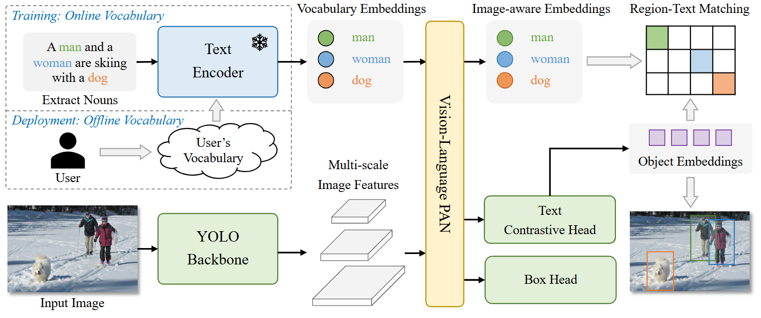
Fig. 1 Overall Architecture of YOLO-World. Compared to traditional YOLO detectors, YOLO-World as an open-vocabulary detector adopts text as input. The Text Encoder first encodes the input text input text embeddings. Then the Image Encoder encodes the input image into multi-scale image features and the proposed RepVL-PAN exploits the multi-level cross-modality fusion for both image and text features. Finally, YOLO-World predicts the regressed bounding boxes and the object embeddings for matching the categories or nouns that appeared in the input text.

Rethinking the Problem: From Category IDs to Region-Text Pairs

To understand YOLO-World, we must first appreciate its fundamental shift in how it formulates the object detection problem.

• Traditional Approach: A standard detector is trained on annotations like \(\Omega = \left\{B_i, c_i\right\}$, where $B_i\) is a bounding box and $c_i$ is a fixed integer category ID (e.g., $1$ for “person,” $2$ for “bicycle,” etc.). The model’s job is to classify a box into one of these fixed numerical categories.

• YOLO-World’s Approach: The paper reformulates the problem. Training annotations are now treated as region-text pairs: \(\Omega = \left\{B_i, t_i\right\}\). Here, $B_i$ is still the bounding box, but $t_i$ is the actual text string that describes the object (e.g., “person,” “a red bicycle,” “dog”).

This seemingly simple change is profound. The task is no longer “classify this box as category #2.” It becomes “find the text description that best matches the visual content of this box.” This reframing makes the problem a direct fit for a vision-language model and is the conceptual key to open-vocabulary detection.

Core Architecture: From YOLO’s PAN to RepVL-PAN

YOLO-World’s main architectural innovation lies in its “neck,” the part of the network that fuses features from the main “backbone.”

The Foundation: Standard YOLO’s Path Aggregation Network (PAN)

The backbone (e.g., Darknet) processes an image and extracts feature maps at different scales. Deeper layers capture high-level semantic information (e.g., “this looks like a face”) but have low spatial resolution, while shallower layers capture fine-grained detail (e.g., edges, textures). These outputs are often called C3, C4, C5, corresponding to feature maps downsampled by 8x, 16x, and 32x respectively.

The neck’s job is to intelligently fuse these multi-scale features. A Path Aggregation Network (PAN) does this in two stages:

1. Top-Down Path: It starts with the most semantic map (C5), upsamples it, and merges it with the next level down (C4). This process repeats, bringing rich semantic context down to the high-resolution maps.
2. Bottom-Up Path: It then takes these newly fused maps and builds a new pyramid from the bottom up, passing strong localization features (edges, textures) from the lower levels back up to the higher ones.

This dual-pathway ensures that all final feature maps have a rich mixture of both high-level semantic meaning and precise low-level spatial detail, which is ideal for detecting objects of various sizes.

The Innovation: YOLO-World’s RepVL-PAN

YOLO-World replaces the standard PAN with a Re-parameterizable Vision-Language PAN (RepVL-PAN). This new neck doesn’t just fuse visual features; it injects textual information directly into the fusion process at every level, making the network “aware” of the words you’re looking for.

Layer Dimensions Deep Dive

Let’s define the dimensions of the feature maps involved, assuming a standard 640x640 input image and a text embedding dimension D=512 (from the CLIP text encoder):

Feature Map	Origin/Purpose	Stride	Spatial Dimensions (H x W)	Channel Dimension (D)
$C3, C4, C5$	Initial visual features from the backbone.	8, 16, 32	80x80, 40x40, 20x20	Varies (e.g., 256, 512, 1024)
$X_l$	Fused visual features inside the PAN, before text guidance.	8, 16, 32	80x80, 40x40, 20x20	512 (Constant)
$P5, P4, P3$	Final text-guided features from RepVL-PAN, sent to the head.	8, 16, 32	80x80, 40x40, 20x20	512 (Constant)

The critical design choice is that the channel dimension D is kept constant (D=512) across all levels of the PAN. This allows a single set of text embeddings to interact consistently with visual features at every scale.

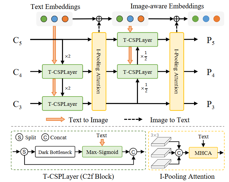
Fig. 2 Illustration of the RepVL-PAN. The proposed RepVLPAN adopts the Text-guided CSPLayer (T-CSPLayer) for injecting language information into image features and the Image Pooling Attention (I-Pooling Attention) for enhancing image-aware text embeddings.

The Mechanisms of Vision-Language Fusion

Text-Guided CSPLayer (T-CSPLayer) in Detail

This is the central component of the RepVL-PAN, responsible for injecting text guidance. For each level l of the feature pyramid, it enhances the visual features $X_l\in \mathbb{R}^{H_l\times W_l\times D}$ using the vocabulary’s text embeddings $W\in \mathbb{R}^{C\times D}$.

\[X^\prime = X_l ⋅ \sigma\left( \max_{j\in{1,\ldots C}} (X_l * W_j^T) \right)\]

This operation can be understood as a two-step “relevance gating” process:

1. Creating the Relevance Map: The model calculates a map that highlights which regions of the image are most relevant to the user’s text prompts. It does this by computing the dot product between the visual features at every position and every word embedding, then taking the maximum score at each position. The result is a single $H_l \times W_l$ map where high values indicate high relevance to any of the vocabulary words.
2. Modulating the Visual Features: This relevance map is passed through a sigmoid function $\sigma$ to become a clean attention gate (with values between 0 and 1). This gate is then multiplied with the original visual features $X_l$. This action preserves features in relevant areas and suppresses them in irrelevant ones, outputting a text-aware feature map $X^\prime$ of the same size $H_l \times W_l \times D$.

Text Contrastive Head & Image-Pooling Attention

After the RepVL-PAN, the detection head proposes bounding boxes. To classify the object within a box, the model uses a sophisticated Image-Pooling Attention mechanism which updates the text embeddings $W$ with visual information from the image region $X$ to make them “image-aware” before computing the final similarity.

\[W^\prime = W + \text{MultiHead-Attention}(W, X,X)\]

How YOLO-World Learns: Training and Loss Functions

The training process is what enables all these mechanisms. Here’s a look at the inputs, outputs, and the loss functions that guide the learning.

Training Inputs and Outputs

• Inputs: A batch of training data, where each sample consists of:
  1. An Image.
  2. A set of Ground-Truth Bounding Boxes ($B_i$).
  3. A corresponding set of Ground-Truth Text Labels ($t_i$) for each box.
• Outputs (Predictions): For each image, the model predicts:
  1. A set of $K$ Predicted Bounding Boxes ($b_k$).
  2. A Predicted Visual Embedding ($e_k$) for the object within each box.

The Combined Loss Function

The total loss $\mathcal{L}(I)$ for an image is a sum of classification and localization losses, intelligently balanced:

\[\mathcal{L}(I) = \mathcal{L}_{con} + \lambda_1 ⋅ (\mathcal{L}_{iou} + \mathcal{L}_{dfl})\]

Let’s break down each component in detail.

$\mathcal{L}_{con}$: The Region-Text Contrastive Loss and the Text Contrastive Head

This is the core classification loss. Its goal is to align the predicted visual embedding $e_k$ of an object with the text embedding $w_j$ of its correct label. This alignment is measured by the Text Contrastive Head, which computes a similarity score $s_{k,j}$.

The Similarity Formula:

\[s_{k,j} = \alpha ⋅ \text{L2-Norm}(e_k) ⋅ \text{L2-Norm}(w_j) + \beta\]

Let’s dissect this formula:

• $e_k$: The visual embedding vector that the model generates for the k-th proposed object box.
• $w_j$: The text embedding vector for the j-th word in the vocabulary, pre-computed by the CLIP encoder.
• $L2-Norm(…)$: This normalizes the vectors, making them unit length. The dot product of two unit vectors is their cosine similarity, which measures the angle between them. A value of 1 means they are perfectly aligned in the semantic space.
• $\alpha$ and $\beta$: These are learnable scaling and shifting parameters that help stabilize the training process.

The Loss Itself: $\mathcal{L}{con}$ is a cross-entropy loss based on these similarity scores. For a predicted box $k$ that is supposed to be a “dog,” the loss encourages the model to maximize the score $s{k, \text{“dog”}}$ while minimizing the scores for all other words like “cat,” “car,” etc. This forces the model to learn a truly discriminative mapping between visual content and text.

$\mathcal{L}{iou}$ and $\mathcal{L}{dfl}$: The Bounding Box Regression Losses

These two standard but crucial losses ensure the predicted bounding boxes are accurate.

• $\mathcal{L}_{iou}$ (Intersection over Union Loss): Penalizes the model for inaccurate boxes by measuring the mismatch in overlap, center point, and aspect ratio.
• $\mathcal{L}_{dfl}$ (Distribution Focal Loss): A more advanced loss that models box coordinates as probability distributions, leading to more precise localization.

The Intelligent Switch: $\lambda_1$

This is a simple but critical controller. For clean, human-annotated data, $\lambda_1$ is 1, enabling all losses. For noisy, pseudo-labeled data with potentially inaccurate boxes, $\lambda_1$ is 0, disabling the localization losses ($\mathcal{L}{iou}$, $\mathcal{L}{dfl}$). This allows the model to learn rich semantics from vast, noisy datasets without corrupting its ability to localize objects accurately.

The Pseudo-Labeling Pipeline

The process of generating pseudo-labels is one of the most critical components that allows YOLO-World to learn from vast, noisy web data. It’s a sophisticated pipeline designed to turn raw image-caption pairs into high-quality training data with accurate bounding boxes and labels.

Let’s break down exactly how it works, step-by-step, as detailed in the paper’s appendix and visualized in Figure 8.

The core idea is to use two different pre-trained models in sequence: a powerful Open-Vocabulary Detector (GLIP) to create initial, “coarse” labels, and a highly reliable Vision-Language Model (CLIP) to act as a “judge” to verify, refine, and filter them.

Imagine we have a single data point from a web-scraped dataset like CC3M: an image and its user-provided caption, for example: “A photograph of a man and a woman skiing.”

Step 1: Extract Key Object Nouns

The first step is to identify the potential objects mentioned in the caption.

• Method: The system uses a simple n-gram algorithm, a standard Natural Language Processing (NLP) technique, to parse the caption and extract the key nouns.
• Example: From “A photograph of a man and a woman skiing,” the algorithm would extract the list of nouns: T = ["man", "woman"].

This gives the system a list of candidate objects to find in the image.

Step 2: Generate Coarse Labels with an Open-Vocabulary Detector (GLIP)

Now, the system needs to find the location of these nouns in the image.

• Method: It uses a powerful, pre-trained open-vocabulary detector. The paper specifies they use GLIP-L. GLIP is given the image and prompted with the list of nouns T.
• Process: GLIP analyzes the image and generates a set of initial proposals, which are essentially bounding boxes with their associated noun label and a confidence score from GLIP itself.
• Example Output: GLIP might produce two proposals:
  1. {box_1, "man", confidence_glip_1}
  2. {box_2, "woman", confidence_glip_2}

At this point, we have initial labels, but they can be noisy. GLIP might have drawn a loose box, or it might have low confidence. The next step is to clean this up.

Step 3: Refine and Filter with a “Judge” Model (CLIP)

This is the most crucial part of the pipeline. The system uses the pre-trained CLIP model, which is exceptionally good at judging the similarity between an image patch and a text description, to verify the coarse labels from GLIP. This refinement happens in several stages:

3a. Compute Region-Text Scores For each proposal from GLIP, the system crops the image region defined by the bounding box and calculates a new similarity score using CLIP.

• Process:
  • Crop the image using box_1.
  • Feed the cropped image of the man and the text “man” into CLIP.
  • CLIP outputs a highly reliable similarity score, let’s call it score_clip_1.
  • Repeat for the woman: crop using box_2, feed the crop and the text “woman” into CLIP to get score_clip_2.

3b. Re-score the Proposals The system now creates a new, more robust confidence score for each proposal by combining the initial confidence from GLIP with the new verification score from CLIP.

• Formula: new_confidence = √(confidence_glip * score_clip)
• Result: This blended score is a much better indicator of the label’s quality than GLIP’s score alone.

3c. Filter at the Region Level Now, the system cleans up the proposals for the image.

• Non-Maximum Suppression (NMS): This standard algorithm removes redundant, highly overlapping boxes for the same object. For example, if GLIP proposed two slightly different boxes for “man,” NMS would keep only the one with the higher score.
• Confidence Thresholding: Any proposal whose new_confidence score is below a certain threshold (the paper uses 0.3) is discarded. This removes low-quality, uncertain labels.

3d. Filter at the Image Level Finally, the system decides if the entire image-caption pair is good enough to be used for training.

• Method: It calculates a final image quality score by combining the average confidence of all its kept pseudo-labels with an overall score of how well the original caption matched the original image (also calculated with CLIP).
• Filtering: If this final image score is too low (below 0.3), the entire image and all its generated pseudo-labels are thrown away. This removes ambiguous images or images with badly mismatching captions.

The Final Output

After this rigorous, multi-stage pipeline, the output is a high-quality, clean pseudo-label. For our example, it would be a tuple like:

{image_file, [ (clean_box_1, "man"), (clean_box_2, "woman") ]}

By repeating this process for hundreds of thousands of image-caption pairs, the authors automatically create a massive and reliable dataset. It is this dataset, with its diverse vocabulary and accurate bounding boxes, that is used to train YOLO-World and grant it the ability to understand and detect a wide array of objects in the wild.

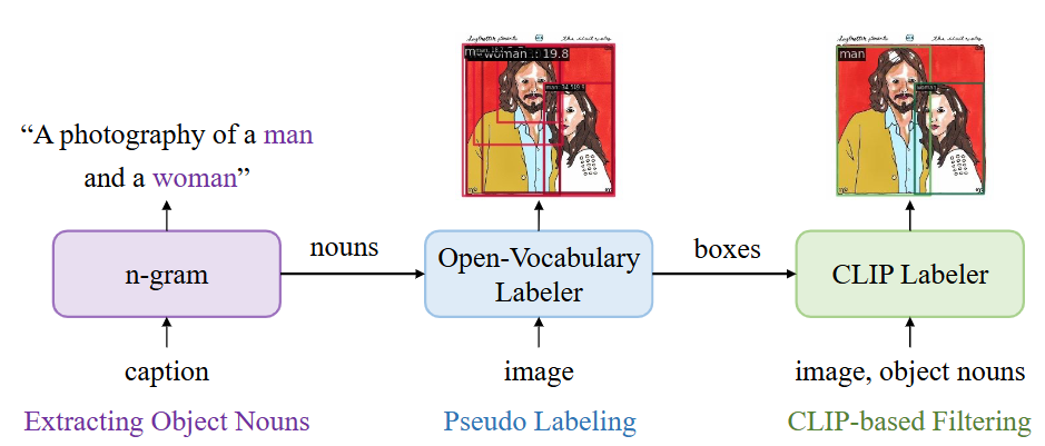
Fig.3 Labeling Pipeline for Image-Text Data We first leverage the simple n-gram to extract object nouns from the captions. We adopt a pre-trained open-vocabulary detector to generate pseudo boxes given the object nouns, which forms the coarse region-text proposals. Then we use a pre-trained CLIP to rescore or relabel the boxes along with filtering.

Of course. Let’s walk through a practical, real-world inference use case to illustrate how YOLO-World is used and why its “Prompt-then-Detect” paradigm is so powerful.

Use Case: Smart Inventory Management in a Retail Store

The Goal: Imagine you are the manager of a large hardware store. You want to automate inventory checks by using a camera to scan shelves and count the items. The problem is that your inventory is constantly changing. One week you might stock a new brand of “cordless drills,” and the next you might need to track “locking pliers.” A traditional object detector would be useless here, as you would need to collect thousands of images and retrain the entire model every time a new product is introduced.

The Tool: You have a computer with a camera connected to it, running an application that uses a pre-trained YOLO-World model.

Here is the step-by-step process of using YOLO-World for this task.

---

Step 1: Define the Vocabulary (The “Prompts”)

This is the first and most important step from the user’s perspective. You decide what you want to find on the shelf right now. You are not limited by what the model was trained on; you are limited only by your imagination.

Let’s say you want to check the stock of specific hand tools on Aisle 4. You create a simple text list of the items you’re interested in:

- phillips head screwdriver
- flat head screwdriver
- claw hammer
- rubber mallet
- safety goggles
- tape measure

Notice the specificity. You aren’t just looking for a “screwdriver”; you are distinguishing between “phillips head” and “flat head.” This is where the power of language comes in.

Step 2: Set the Vocabulary in the Application

This is the “Prompt-then-Detect” part of the process. The application has a simple interface (e.g., a text box or a configuration file) where you provide your list of prompts.

• Behind the Scenes (Offline Vocabulary Encoding): This is the first action the YOLO-World system takes. It does this once when you set the vocabulary, before it even looks at an image.
  1. The list of six strings is fed into the frozen CLIP Text Encoder.
  2. The text encoder converts each phrase into a 512-dimensional vector embedding.
  3. The output is a small matrix W of size 6 x 512 (6 nouns, 512 dimensions each). This matrix is the “offline vocabulary” and is stored in memory. This step is extremely fast.

Step 3: Run Inference on the Live Camera Feed

You now point the camera at the shelf on Aisle 4. The application begins processing the video stream in real-time.

• Behind the Scenes (Real-Time Detection): For each frame from the camera, the following happens instantly:

  1. Visual Processing: The image frame is fed into the YOLO-World model’s backbone and its RepVL-PAN. The network generates text-aware feature pyramids, as described in the tutorial. It has a general idea of where “things” are.

  2. Class-Agnostic Object Proposal: The detection head scans the feature pyramids and identifies regions that have high “objectness.” It draws class-agnostic bounding boxes around these regions. At this stage, it has found, for example, a hammer-shaped object and a screwdriver-shaped object, but it has not yet named them.

  3. Matching and Classification (The Core Logic): For each proposed bounding box, the model performs the crucial matching step:

     • It extracts the visual features from within the box and computes its visual embedding, e_k.
     • It then calculates the cosine similarity between this single visual embedding e_k and all six of the text embeddings stored in your vocabulary matrix W.
     • For the hammer-shaped object, the similarity scores might look like this:
       • similarity(e_k, "claw hammer") -> 0.92 (Very high)
       • similarity(e_k, "rubber mallet") -> 0.65 (Similar, but less so)
       • similarity(e_k, "tape measure") -> 0.15 (Very low)
       • …and so on for the other prompts.
     • The model assigns the label with the highest similarity score (“claw hammer”) to the bounding box.

Step 4: View the Results

The application displays the video feed on your screen. The output is exactly what you need:

• A tight bounding box is drawn around each of the tools you specified.
• Each box is labeled with the correct text from your list: “claw hammer,” “phillips head screwdriver,” “safety goggles,” etc.
• A confidence score (e.g., 0.92) is displayed next to each label.

The application can now easily count the number of boxes for each label to give you a real-time inventory count for that shelf.

The Game-Changing Advantage

The next day, a new shipment of “ball-peen hammers” arrives.

• With a Traditional Detector: You would be stuck. Your model has never seen this item, and you’d have to start a weeks-long process of data collection and retraining.
• With YOLO-World: You simply add "ball-peen hammer" to your text list in the application’s config. The model instantly knows how to find it. Because it understands language, it can differentiate the visual features of a “ball-peen hammer” (a rounded head) from a “claw hammer” (a forked claw) based solely on the text description you provided.

This use case demonstrates how YOLO-World moves object detection from a rigid, pre-programmed task to a dynamic, flexible, and interactive process.

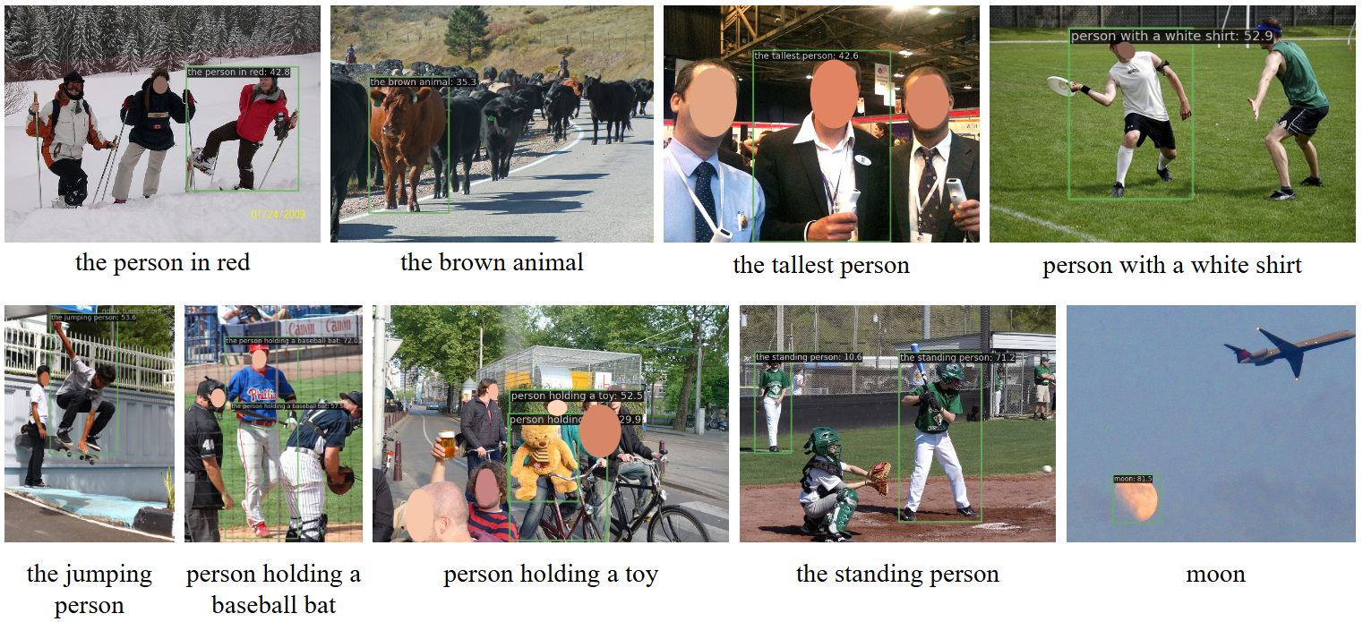
Fig. 4 Visualization Results on Referring Object Detection. We explore the capability of the pre-trained YOLO-World to detect objects with descriptive noun phrases. Images are obtained from COCO val2017.

Reference

For further details, please refer to the original research paper:

• Cheng, T., Song, L., Ge, Y., Liu, W., Wang, X., & Shan, Y. (2024). YOLO-World: Real-Time Open-Vocabulary Object Detection. arXiv preprint arXiv:2401.17270. Available at: https://arxiv.org/abs/2401.17270