ViLBERT: Pretraining Task-Agnostic Visiolinguistic Representations
This tutorial breaks down the ViLBERT model, a seminal work in vision-and-language pre-training.
1. The Intuition: What Problem Does ViLBERT Solve?
Before ViLBERT, models for tasks like Visual Question Answering (VQA) or Image Captioning were often trained from scratch for that specific task. This required large, task-specific labeled datasets and didn’t leverage knowledge from other related tasks.
The core idea of ViLBERT is inspired by the success of BERT in Natural Language Processing (NLP). BERT is pre-trained on a massive amount of text data with self-supervised objectives (like guessing masked words). This allows it to learn a deep, general-purpose understanding of language, which can then be quickly fine-tuned for various downstream tasks (like sentiment analysis or question answering).
ViLBERT extends this “pre-train and fine-tune” paradigm to vision-and-language. The goal is to create a model that learns a fundamental, shared representation of visual and textual concepts from large, unlabeled datasets of image-text pairs. This pre-trained model can then be adapted to solve a wide range of vision-and-language tasks with minimal additional training.
The key innovation is how it processes both modalities. Instead of just mushing the image and text information together from the start, ViLBERT uses a two-stream architecture. Imagine two separate “experts”: one that reads text and one that looks at images. They first process their own input independently and then communicate back and forth to build a joint understanding.
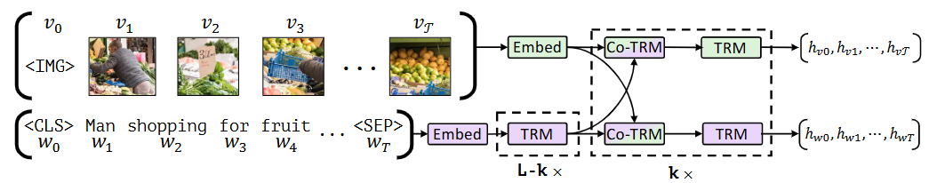
Fig.1 ViLBERT model consists of two parallel streams for visual (green) and linguistic (purple) processing that interact through novel co-attentional transformer layers. This structure allows for variable depths for each modality and enables sparse interaction through co-attention. Dashed boxes with multiplier subscripts denote repeated blocks of layers.
2. Model Architecture
ViLBERT consists of two parallel BERT-style Transformer networks—one for processing text (the linguistic stream) and one for processing regions in an image (the visual stream). These streams interact through a series of novel “co-attentional transformer layers.”
a. Overall Structure
- Two-Stream Design: A linguistic stream and a visual stream.
- Linguistic Stream: A standard Transformer encoder.
- Visual Stream: A Transformer encoder that operates on image region features.
- Co-Attentional Layers: Special layers that allow information exchange between the two streams.
b. Input Representation
- Textual Input: A sentence is turned into a sequence of vectors, where each vector represents a word or sub-word. The final dimension for each vector in the textual stream is 768.
- Visual Input: An image is broken down into a set of important regions, and each region is turned into a vector. The final dimension for each vector in the visual stream is 1024.
Textual Input Explained
The textual input processing is almost identical to the original BERT model. The final input embedding for each token is a sum of three distinct embeddings.
Input: A raw text sentence, e.g., “A man is playing guitar.“
Step 1: Tokenization
The sentence is first broken down into “tokens.” ViLBERT uses a method called WordPiece tokenization, which can break down uncommon words into smaller, more manageable sub-words. Special tokens are also added:
[CLS]: This token is always placed at the beginning of the sequence. Its final hidden state is often used as a summary of the entire sentence for classification tasks.[SEP]: This token signifies the end of a sentence.
Example:
"A man is playing guitar." becomes [CLS], A, man, is, play, ##ing, guitar, [SEP]
Step 2: Creating the Final Input Embeddings: For each token in the sequence, its final input vector is the sum of three components:
A. Token Embeddings:
- What it is: A learned vector that represents the token’s meaning.
- How it’s generated: The model has a large vocabulary (e.g., 30,000 words/sub-words). The token embedding is simply looked up from an embedding matrix of size
(vocabulary_size, 768). Each token corresponds to a unique 768-dimensional vector.
B. Positional Embeddings:
- What it is: A vector that encodes the position of the token in the sequence.
- Why it’s needed: The Transformer architecture itself has no inherent sense of order. Without positional information, “man bites dog” and “dog bites man” would look the same to the model.
- How it’s generated: The model learns a unique 768-dimensional vector for each possible position (e.g., position 0, position 1, up to a maximum sequence length). This learned vector is then added to the token embedding.
C. Segment Embeddings:
- What it is: A vector that identifies which sentence a token belongs to.
- Why it’s needed: For tasks that involve two sentences (like Question Answering), this helps the model distinguish between Sentence A (the question) and Sentence B (the context).
- How it’s generated: All tokens in the first sentence get a learned “Segment A” embedding, and all tokens in the second get a “Segment B” embedding. For single-sentence tasks, all tokens simply get the “Segment A” embedding.
Final Textual Input:
Final Token Vector = Token Embedding + Positional Embedding + Segment Embedding
This process results in a sequence of vectors of shape (Sequence Length, 768).
Visual Input Explained
This is where ViLBERT introduces its novel approach. The goal is the same—create a sequence of vectors—but the source is an image.
Input: A raw image.
Step 1: From Image to Object Regions
ViLBERT doesn’t treat the image as a single entity. It first identifies the most important or “salient” regions within it.
- How it’s done: A powerful, pretrained object detection model, Faster R-CNN, is used. This model was trained on the large-scale Visual Genome dataset, so it’s very good at identifying a wide variety of objects and their locations.
- The Output: The Faster R-CNN proposes a set of bounding boxes for potential objects in the image. The ViLBERT authors filter these, keeping between 10 to 36 of the highest-confidence regions for each image.
Now, for each of these regions, we need to create an embedding.
Step 2: Creating the Final Image Region Embeddings
Similar to the text input, the final vector for each image region is a sum of two components:
A. Image Region Feature (The “Token” Embedding for Images):
- What it is: A vector that represents the visual appearance of what’s inside a region’s bounding box.
- How it’s generated: For each bounding box, the corresponding features from the Faster R-CNN’s internal convolutional layers are extracted. These features are then “mean-pooled” to produce a single, fixed-size vector. This vector captures the visual essence of the object (e.g., “fluffy,” “brown,” “has four legs”).
- Dimension: This feature vector is 1024-dimensional.
- Special
[IMG]Token: An additional “token” is created to represent the entire image. Its feature is the mean of all the other region features. This serves a similar purpose to the[CLS]token in the text stream.
B. Positional Embedding for Images (The “Where” Information):
- What it is: A vector that encodes the spatial location and size of the region within the image.
- Why it’s needed: The model needs to know where objects are. Is the man on the grass or next to the car? This spatial context is crucial.
- How it’s generated:
- A 5-dimensional vector is created for each region’s bounding box:
x1, y1: The coordinates of the top-left corner, normalized to be between 0 and 1.x2, y2: The coordinates of the bottom-right corner, normalized.w*h: The fraction of the total image area that the bounding box covers.
- This 5-dimensional vector is then fed through a linear layer (a learned matrix multiplication) to project it into a 1024-dimensional vector, matching the dimension of the image region feature.
- A 5-dimensional vector is created for each region’s bounding box:
Final Visual Input:
Final Region Vector = Image Region Feature + Projected Positional Embedding
This process results in a sequence of vectors of shape (Number of Regions, 1024).

Fig. 2 Co-attention mechanism: By exchanging key-value pairs in multi-headed attention, this structure enables vision-attended language features to be incorporated into visual representations (and vice versa).
So, the input to the visual stream is a sequence of region features, and the input to the linguistic stream is a sequence of word embeddings.
c. Co-Attentional Transformer Layer
This is the core of ViLBERT. A standard Transformer layer consists of a Multi-Head Self-Attention module followed by a Feed-Forward Network. In ViLBERT’s co-attentional layers, the attention mechanism is modified to allow one stream to attend to the other.
Let’s denote the hidden states from the visual stream as $H_V$ and from the linguistic stream as $H_L$.
A single co-attentional transformer block works as follows:
-
Multi-Head Co-Attention:
- The visual stream calculates its new representations by attending to the language stream. The queries ($Q_V$) come from the visual stream, but the keys ($K_L$) and values ($V_L$) come from the linguistic stream. This lets each image region “ask” the text: “Which words are most relevant to me?”
- Simultaneously, the linguistic stream attends to the visual stream. The queries ($Q_L$) come from the linguistic stream, and the keys ($K_V$) and values ($V_V$) come from the visual stream. This lets each word “ask” the image: “Which regions are most relevant to me?”
-
Feed-Forward Networks: After the co-attention step, the updated hidden states in each stream are passed through their own separate Feed-Forward Networks (FFN), just like in a standard Transformer.
This block is stacked multiple times, allowing for deep and iterative fusion of information.
3. Mathematics of Co-Attention
The fundamental building block is Scaled Dot-Product Attention:
\[\text{Attention}(Q, K, V) = \text{softmax}\left(\frac{QK^T}{\sqrt{d_k}}\right)V\]where $Q$ is the query, $K$ is the key, $V$ is the value, and $d_k$ is the dimension of the key.
In a Co-Attentional Layer, let $H_L^{(i-1)}$ and $H_V^{(i-1)}$ be the outputs of the previous layer for the linguistic and visual streams, respectively.
The new intermediate hidden states ($H^\prime_{L}$ and $H^\prime_{V}$) are calculated via multi-head co-attention:
\[H^\prime_{L} = \text{Co-Attention}(Q=H_L^{(i-1)}, K=H_V^{(i-1)}, V=H_V^{(i-1)})\] \[H^\prime_{V} = \text{Co-Attention}(Q=H_V^{(i-1)}, K=H_L^{(i-1)}, V=H_L^{(i-1)})\]After attention, Layer Normalization and residual connections are applied, followed by a standard Position-wise Feed-Forward Network (FFN) for each stream separately to get the final outputs $H_L^{(i)}$ and $H_V^{(i)}$.
\[H_L^{(i)} = \text{FFN}_L(\text{LayerNorm}(H_L^{(i-1)} + H^\prime_{L}))\] \[H_V^{(i)} = \text{FFN}_V(\text{LayerNorm}(H_V^{(i-1)} + H^\prime_{V}))\]The visual stream has a hidden dimension of 1024, and the textual stream has a hidden dimension of 768. You cannot directly perform operations like dot products or element-wise addition between vectors of different sizes.
The solution is elegant and simple: dedicated linear projections for cross-modal interaction.
Before the attention mechanism calculates the scores, ViLBERT uses separate nn.Linear layers (simple matrix multiplications) to project the Query, Key, and Value vectors into compatible dimensions. The key is that these projection layers are different for each interaction direction.
Let’s break it down into the two directions of co-attention.
Case 1: Text Attending to Image
In this case, the textual stream is the one asking the questions (“Queries”), and it’s looking at the visual stream for context (“Keys” and “Values”). The final output must be 768-dimensional so it can be added back to the original text stream via the residual connection.
- Goal: Update the text representations.
- Query (Q) Source: Text Stream (hidden size 768)
- Key (K) Source: Image Stream (hidden size 1024)
- Value (V) Source: Image Stream (hidden size 1024)
Here’s how the dimensions are handled:
- Generate Query (Q) for Text: A linear layer projects the 768-dim text input into a 768-dim query vector.
W_Q_text: A weight matrix of size(768, 768).
- Generate Key (K) for Image: A linear layer projects the 1024-dim image input into a 768-dim key vector. This is the crucial step.
W_K_image: A weight matrix of size(1024, 768).
- Generate Value (V) for Image: A linear layer projects the 1024-dim image input into a 768-dim value vector.
W_V_image: A weight matrix of size(1024, 768).
Now, the attention can be calculated:
Attention(Q_text, K_image, V_image)
- The dot product between
Q_text(768-dim) andK_image(768-dim) is now valid. - The output of the attention mechanism will have the same dimension as the Value vector,
V_image, which is 768. - This 768-dim output can now be correctly added back to the original 768-dim text stream input.
Case 2: Image Attending to Text
Now we flip it. The visual stream is asking the questions (“Queries”), and it’s looking at the textual stream for context (“Keys” and “Values”). The final output must be 1024-dimensional to be compatible with the visual stream.
- Goal: Update the image representations.
- Query (Q) Source: Image Stream (hidden size 1024)
- Key (K) Source: Text Stream (hidden size 768)
- Value (V) Source: Text Stream (hidden size 768)
Here’s how the dimensions are handled in this direction:
- Generate Query (Q) for Image: A linear layer projects the 1024-dim image input into a 1024-dim query vector.
W_Q_image: A weight matrix of size(1024, 1024).
- Generate Key (K) for Text: A linear layer projects the 768-dim text input into a 1024-dim key vector.
W_K_text: A weight matrix of size(768, 1024).
- Generate Value (V) for Text: A linear layer projects the 768-dim text input into a 1024-dim value vector.
W_V_text: A weight matrix of size(768, 1024).
Now, the attention can be calculated:
Attention(Q_image, K_text, V_text)
- The dot product between
Q_image(1024-dim) andK_text(1024-dim) is now valid. - The output of the attention mechanism will have the same dimension as the Value vector,
V_text, which is 1024. - This 1024-dim output can be correctly added back to the original 1024-dim image stream input.
Analogy
Think of these linear projections as specialized adaptors or translators.
Each stream maintains its own “native” dimensionality (768 for text, 1024 for vision). When they need to interact, they use a set of learned translators (the W matrices) to convert the incoming information into a dimension that is compatible for the operation, ensuring that the final output is in the native dimension of the stream being updated. This allows for rich interaction without forcing both modalities into a single, potentially suboptimal, shared dimension.
4. Pre-training Tasks and Loss Functions
ViLBERT’s pre-training is driven by two main objectives, which break down into three distinct loss functions. These losses are designed to work together to teach the model a fundamental and general-purpose understanding of how vision and language connect.
The total pre-training loss is a simple sum of these three individual loss components:
\[\mathcal{L}_{Pre} = \mathcal{L}_{MLM} + \mathcal{L}_{MRM} + \mathcal{L}_{ALIGN}\]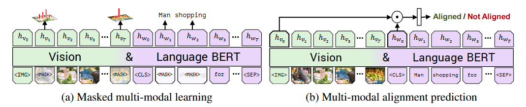
Fig. 3 ViLBERT is trained on the Conceptual Captions [24 ] dataset under two training tasks to learn visual grounding. In masked multi-modal learning, the model must reconstruct image region categories or words for masked inputs given the observed inputs. In multi-modal alignment prediction, the model must predict whether or not the caption describes the image content.
Let’s break down each one in detail.
Objective 1: Masked Multi-modal Modeling
The goal of this objective is to teach the model to use context from both the visual and textual streams to fill in the blanks in each modality. This is analogous to the Masked Language Model task in the original BERT.
1. Masked Language Modeling Loss ($\mathcal{L}_{MLM}$)
-
The Goal: To predict words that have been randomly hidden (masked) in the input text. This forces the model to learn rich contextual representations of language, but with the added twist that it can now use visual information to help its prediction. For instance, if the text is
[CLS] A person is riding a [MASK] on the water. [SEP]and the image contains a jet ski, the model should learn to predict “jet ski” by looking at the image. -
The Process:
- About 15% of the text tokens in a sentence are randomly selected for masking.
- Of these selected tokens:
- 80% are replaced with a special
[MASK]token. - 10% are replaced with a random word from the vocabulary.
- 10% are left unchanged.
- 80% are replaced with a special
- The model must then predict the original token for every masked position.
-
The Math (Cross-Entropy Loss): The output for each masked token is a probability distribution over the entire vocabulary, calculated using a softmax function. The loss is the standard Cross-Entropy Loss, which measures how different the model’s predicted distribution is from the “true” distribution (which is a one-hot vector where the correct word is 1 and all others are 0).
For a single masked token, the loss is:
\[\mathcal{L}_{MLM} = - \sum_{i=1}^{V} y_i \log(\hat{y}_i)\]Where:
- $V$ is the size of the vocabulary.
- $y_i$ is 1 if word
iis the correct word, and 0 otherwise. - $\hat{y}_i$ is the model’s predicted probability that the word is
i.
2. Masked Region Modeling Loss ($\mathcal{L}_{MRM}$)
-
The Goal: To predict the semantic content of image regions that have been hidden (masked). This is the visual equivalent of MLM. It forces the model to use the textual context and the surrounding visual context to infer what is missing from the image.
-
The Process:
- About 15% of the image regions are randomly selected for masking.
- 90% of the time, the feature vector for a masked region is completely replaced by zeros. 10% of the time, it’s left unchanged.
- Instead of trying to predict the exact, high-dimensional feature vector back (which is too difficult), the model is trained to predict a distribution over possible object classes for that region.
- The “ground truth” for this prediction is the class distribution produced by the pre-trained object detector (Faster R-CNN) that was used to generate the regions initially.
-
The Math (Kullback-Leibler Divergence Loss): The loss function measures the “distance” between the model’s predicted probability distribution and the ground truth distribution from the object detector. The perfect tool for this is the Kullback-Leibler (KL) Divergence.
\[\mathcal{L}_{MRM} = D_{KL}(P_{detector} || P_{model})\]Where $D \left( P || Q \right)= \sum_{i=1}^{C} p(i) \log\left(\frac{p(i)}{q(i)}\right)$ and :
- $C$ is the number of possible object classes.
- $p(i)$ is the ground truth probability for class
i(from the object detector). - $q(i)$ is ViLBERT’s predicted probability for class
i.
Objective 2: Multi-modal Alignment Prediction
The goal of this objective is to teach the model to understand whether an entire image and a sentence are a match at a holistic level.
3. Alignment Prediction Loss ($\mathcal{L}_{ALIGN}$)
-
The Goal: To look at a pair of (Image, Caption) and predict whether the caption is the correct description for the image. This teaches the model to learn a global correspondence between the visual scene and the textual narrative.
-
The Process:
- Positive Examples: The model is fed a correct (Image A, Caption A) pair. The target label is
1(Aligned). - Negative Examples: The model is fed an incorrect (Image A, Caption B) pair, where Caption B is from a random different image. The target label is
0(Not Aligned). - The model’s prediction is made by taking the final representation of the
[IMG]token (from the visual stream) and the[CLS]token (from the textual stream), multiplying them together, and passing the result through a simple linear classifier to get a single probability score.
- Positive Examples: The model is fed a correct (Image A, Caption A) pair. The target label is
-
The Math (Binary Cross-Entropy Loss): Since this is a binary classification problem (Aligned or Not Aligned), the loss function is the standard Binary Cross-Entropy (BCE) Loss.
\[\mathcal{L}_{ALIGN} = - [y \log(\hat{y}) + (1-y) \log(1-\hat{y})]\]Where:
- $y$ is the true label (1 for aligned, 0 for not aligned).
- $\hat{y}$ is the model’s predicted probability of the pair being aligned.
5. Fine-Tuning and Inference
Of course. After ViLBERT is pre-trained on a massive, general-purpose dataset, its real power is unlocked by fine-tuning it for specific “downstream” tasks. Fine-tuning involves taking the pre-trained model, adding a small task-specific classification head, and then continuing the training on a smaller, task-specific dataset.
Here’s a breakdown of the four main downstream tasks from the paper, explaining how ViLBERT is adapted for each.
1. Visual Question Answering (VQA)
The Task
Given an image and a question about that image, the model must provide an accurate answer. This is an open-ended prediction problem, but it’s typically framed as a classification task over a set of possible answers.
- Example:
- Image: A photo of a person on a sunny beach holding a yellow surfboard.
- Question: “What is the person holding?”
- Expected Answer: “surfboard”
Input-Output Training Pair
- Input: An (Image, Question) pair.
- Output: A “soft score” for each possible answer in the dataset’s answer vocabulary (e.g., the VQA dataset has 3,129 common answers). The score reflects how many human annotators gave that answer. For example, if 9/10 people said “surfboard” and 1/10 said “board”, the target output would be
{surfboard: 0.9, board: 0.3, ...}(the scores are not probabilities and don’t sum to 1).
Fine-Tuning Process
- Model Input: The image is fed into the visual stream, and the question is fed into the linguistic stream.
- Combining Information: The final hidden state of the
[IMG]token (representing the whole image) and the[CLS]token (representing the question) are extracted from the two streams. - Classification Head: These two vectors are combined with an element-wise product (
h_IMG * h_CLS). This resulting vector, which now contains joint information from both modalities, is fed into a new, small Multi-Layer Perceptron (MLP). This MLP is the task-specific head. - Loss Function: The MLP outputs a score for every possible answer. This is trained using a Binary Cross-Entropy Loss against the soft target scores for all answers. This allows the model to predict multiple plausible answers.
Inference (Getting a Prediction)
- Feed the new image and question into the fine-tuned model.
- Get the output scores from the final MLP layer.
- Apply a
softmaxfunction to these scores to turn them into a probability distribution. - The final answer is the one with the highest probability.
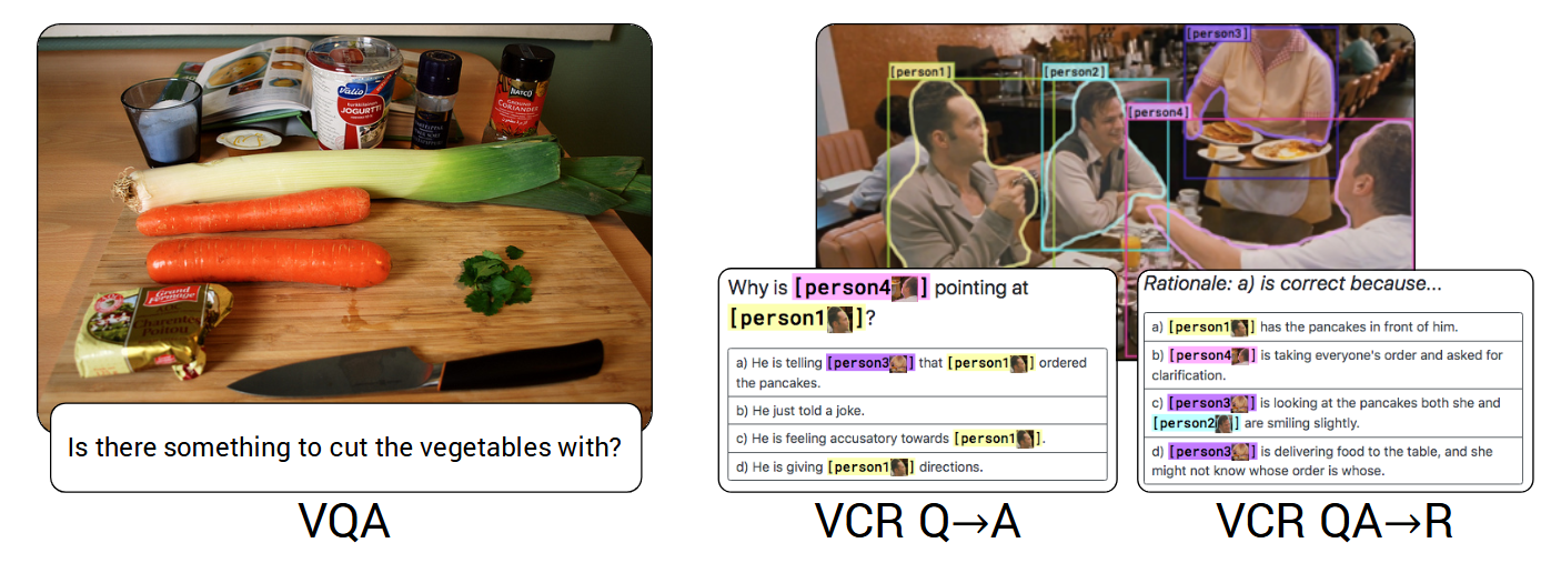
Fig. 4 Examples for each vision-and-language task ViLBERT is transferred to in experiments.
2. Visual Commonsense Reasoning (VCR)
The Task
This is a more advanced, multiple-choice QA task that requires commonsense reasoning. For a given question, the model must not only choose the correct answer but also the correct rationale (justification) for that answer.
- Example:
- Image: A photo of four people at a dinner table, where person
[c]is laughing. - Question: “Why is person
[c]laughing?” - Answer Choices: (a) Because person
[a]is singing., (b) Because person[b]just told a joke., etc.
- Image: A photo of four people at a dinner table, where person
Input-Output Training Pair
- Input: An (Image, Question, List of 4 Answer Choices).
- Output: The index of the correct answer choice (e.g.,
1for choice b).
Fine-Tuning Process
This task requires a clever setup to handle the multiple-choice format.
- Model Input: For a single question with four answer choices (A, B, C, D), you create four separate input pairs:
- Pair 1: (Image, “Question text” + “Answer A text”)
- Pair 2: (Image, “Question text” + “Answer B text”)
- Pair 3: (Image, “Question text” + “Answer C text”)
- Pair 4: (Image, “Question text” + “Answer D text”)
- Combining Information: Each of these four pairs is passed through ViLBERT to get a final joint representation (
h_IMG * h_CLS). - Classification Head: A new linear layer is added that takes this joint vector and outputs a single “correctness” score for each pair. You now have four scores, one for each answer choice.
- Loss Function: A
softmaxis applied across these four scores to create a probability distribution. The model is then trained with a standard Cross-Entropy Loss to maximize the probability of the correct choice.
Inference
- Just like in fine-tuning, create four input pairs for the image, question, and each of the four answer choices.
- Pass all four through the model to get four scores.
- The predicted answer is the choice that received the highest score.
3. Referring Expressions
The Task
Given an image and a textual description of a specific object, the model must locate that object by outputting its bounding box.
- Example:
- Image: A photo with several animals.
- Description: “the brown dog sitting on the right”
- Expected Output: The bounding box coordinates
[x, y, width, height]for that specific dog.
Input-Output Training Pair
- Input: An (Image, Text Description) pair. The image is pre-processed into a set of region proposals (e.g., 36 candidate bounding boxes from a detector).
- Output: For each proposed region, a binary label indicating if it’s the correct one (i.e., if its Intersection-over-Union (IoU) with the ground-truth box is > 0.5).
Fine-Tuning Process
This is different because the goal is to score regions, not the whole image.
- Model Input: The image (as a set of region proposals) is fed to the visual stream. The text description is fed to the linguistic stream.
- Combining Information: For each image region
i, we take its final hidden state vectorh_vi. - Classification Head: A new linear layer is added that takes each region’s vector
h_viand outputs a single “matching score”. This score represents how well that region matches the text description. - Loss Function: Since each region is being classified as a “match” or “not a match,” the model is trained with a Binary Cross-Entropy Loss over all the proposed regions.
Inference
- Pass the new image and text description through the fine-tuned model.
- Calculate the matching score for every proposed region.
- We can simply take the maximum score on the output.
- The final output is the bounding box of the region that received the highest score. The bounding box is retrieved from the output of the initial Region Proposal Network( we created positional embeddings from).
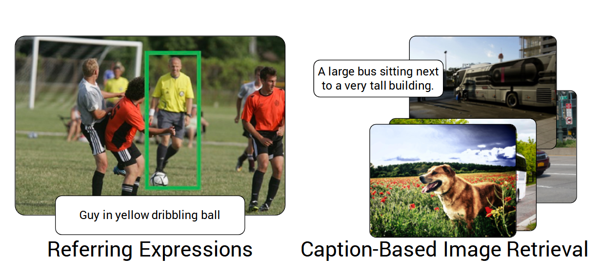
Fig. 5 Examples for each vision-and-language task ViLBERT is transferred to in experiments.
4. Caption-Based Image Retrieval
The Task
Given a query caption, search through a large collection of images and return the one that best matches the caption.
- Example:
- Query Caption: “A person skiing down a snowy mountain.”
- Expected Output: The image from the database that depicts this scene.
Input-Output Training Pair
- Input: An (Image, Caption) pair.
- Output: A binary label:
1if they are a correct pair,0otherwise.
Fine-Tuning Process
This is almost identical to the multi-modal alignment pre-training task.
- Model Input: An (Image, Caption) pair.
- Combining Information: Get the final
[IMG]and[CLS]representations and combine them via element-wise product. - Classification Head: A new linear layer takes this joint vector and outputs a single alignment score.
- Loss Function: The model is trained with Binary Cross-Entropy Loss on the alignment score, using positive (correctly matched) and negative (mismatched) pairs.
Inference
- Pre-computation: Pass the single query caption through the linguistic stream of ViLBERT and store its final
[CLS]vector. This only needs to be done once. - Scoring: For every image in the database, pass it through the visual stream to get its
[IMG]vector. Calculate the alignment score between the stored caption vector and each image vector. - Ranking: Rank all images in the database from highest to lowest score.
- The final output is the top-ranked image (or top-k images).
Fig. 6 Qualitative examples of sampled image descriptions from a ViLBERT model after our pretraining tasks, but before task-specific fine-tuning.
6. Sample Code Snippet
import torch
import torch.nn as nn
import torch.nn.functional as F
import math

class MultiHeadCoAttention(nn.Module):
    """
    A module for multi-head co-attention between two streams.
    """
    def __init__(self, d_model, num_heads):
        super().__init__()
        assert d_model % num_heads == 0
        self.d_k = d_model // num_heads
        self.num_heads = num_heads
        self.d_model = d_model

        self.query_proj = nn.Linear(d_model, d_model)
        self.key_proj = nn.Linear(d_model, d_model)
        self.value_proj = nn.Linear(d_model, d_model)
        self.out_proj = nn.Linear(d_model, d_model)

    def forward(self, query_stream, key_value_stream, mask=None):
        """
        Args:
            query_stream (Tensor): Shape (batch_size, seq_len_q, d_model)
            key_value_stream (Tensor): Shape (batch_size, seq_len_kv, d_model)
            mask (Tensor): Optional mask.
        """
        batch_size = query_stream.size(0)

        # 1. Linear projections
        Q = self.query_proj(query_stream)  # (B, seq_len_q, D)
        K = self.key_proj(key_value_stream)  # (B, seq_len_kv, D)
        V = self.value_proj(key_value_stream)  # (B, seq_len_kv, D)

        # 2. Reshape for multi-head attention
        Q = Q.view(batch_size, -1, self.num_heads, self.d_k).transpose(1, 2) # (B, H, seq_len_q, d_k)
        K = K.view(batch_size, -1, self.num_heads, self.d_k).transpose(1, 2) # (B, H, seq_len_kv, d_k)
        V = V.view(batch_size, -1, self.num_heads, self.d_k).transpose(1, 2) # (B, H, seq_len_kv, d_k)

        # 3. Scaled dot-product attention
        scores = torch.matmul(Q, K.transpose(-2, -1)) / math.sqrt(self.d_k) # (B, H, seq_len_q, seq_len_kv)
        if mask is not None:
            scores = scores.masked_fill(mask == 0, -1e9)

        attn_weights = F.softmax(scores, dim=-1)
        context = torch.matmul(attn_weights, V) # (B, H, seq_len_q, d_k)

        # 4. Concatenate heads and final linear layer
        context = context.transpose(1, 2).contiguous().view(batch_size, -1, self.d_model) # (B, seq_len_q, D)
        output = self.out_proj(context)

        return output

class PositionwiseFeedForward(nn.Module):
    "Implements FFN equation."
    def __init__(self, d_model, d_ff, dropout=0.1):
        super().__init__()
        self.w_1 = nn.Linear(d_model, d_ff)
        self.w_2 = nn.Linear(d_ff, d_model)
        self.dropout = nn.Dropout(dropout)
        self.activation = nn.GELU()

    def forward(self, x):
        return self.w_2(self.dropout(self.activation(self.w_1(x))))

class CoAttentionalTransformerLayer(nn.Module):
    def __init__(self, d_model=768, num_heads=12, d_ff=3072, dropout=0.1):
        super().__init__()

        # Co-Attention Modules
        self.visn_co_attn = MultiHeadCoAttention(d_model, num_heads)
        self.lang_co_attn = MultiHeadCoAttention(d_model, num_heads)

        # Feed-Forward Networks
        self.visn_ffn = PositionwiseFeedForward(d_model, d_ff, dropout)
        self.lang_ffn = PositionwiseFeedForward(d_model, d_ff, dropout)

        # Layer Normalization
        self.norm1_v = nn.LayerNorm(d_model)
        self.norm1_l = nn.LayerNorm(d_model)
        self.norm2_v = nn.LayerNorm(d_model)
        self.norm2_l = nn.LayerNorm(d_model)

        self.dropout = nn.Dropout(dropout)

    def forward(self, visn_input, lang_input, visn_mask=None, lang_mask=None):
        """
        Args:
            visn_input (Tensor): Visual features, (B, num_regions, D)
            lang_input (Tensor): Language features, (B, seq_len, D)
        """
        # --- Co-Attention Block ---
        # Vision stream attends to language stream
        visn_co_attn_out = self.visn_co_attn(query_stream=visn_input, key_value_stream=lang_input, mask=lang_mask)
        visn_attended = self.norm1_v(visn_input + self.dropout(visn_co_attn_out))

        # Language stream attends to vision stream
        lang_co_attn_out = self.lang_co_attn(query_stream=lang_input, key_value_stream=visn_input, mask=visn_mask)
        lang_attended = self.norm1_l(lang_input + self.dropout(lang_co_attn_out))

        # --- Feed-Forward Block ---
        # FFN for vision stream
        visn_ffn_out = self.visn_ffn(visn_attended)
        visn_output = self.norm2_v(visn_attended + self.dropout(visn_ffn_out))

        # FFN for language stream
        lang_ffn_out = self.lang_ffn(lang_attended)
        lang_output = self.norm2_l(lang_attended + self.dropout(lang_ffn_out))

        return visn_output, lang_output

# Example Usage
if __name__ == '__main__':
    # Dummy inputs
    batch_size = 4
    num_regions = 36  # e.g., from Faster R-CNN
    seq_len = 20
    d_model = 768

    visn_feats = torch.randn(batch_size, num_regions, d_model)
    lang_feats = torch.randn(batch_size, seq_len, d_model)

    # Instantiate one layer
    co_attn_layer = CoAttentionalTransformerLayer(d_model=d_model)

    # A full ViLBERT model would stack these layers
    visn_out, lang_out = co_attn_layer(visn_feats, lang_feats)

    print("Output visual features shape:", visn_out.shape)
    print("Output language features shape:", lang_out.shape)
7. Reference
The original paper provides all the in-depth details of the model, experiments, and results.
- Title: ViLBERT: Pretraining Task-Agnostic Visiolinguistic Representations for Vision-and-Language Tasks
- Authors: Jiasen Lu, Dhruv Batra, Devi Parikh, Stefan Lee
- Conference: Advances in Neural Information Processing Systems (NeurIPS) 2019
- Link: https://arxiv.org/abs/1908.02265