Comprehensive Guide to Vision Transformers (ViTs)
Table of Contents
- Introduction to Vision Transformers
- Positional Encoding
- Embedding Layers and Class Token
- Transformer Blocks in Sequential Order
- Complete Transformer Block Code
- End-to-End Vision Transformer Model
- Classification Example Using Vision Transformers
- Drawbacks of Attention Modules
- Overcoming Expensive Attention Modules
- Conclusion
1. Introduction to Vision Transformers
Overview
Vision Transformers (ViTs) apply the Transformer architecture, originally designed for natural language processing (NLP), to computer vision tasks like image classification. ViTs treat an image as a sequence of patches (akin to words in a sentence) and process them using Transformer encoders.
Key Components
- Patch Embedding: Divides the image into patches and projects them into a vector space.
- Positional Encoding: Adds positional information to patch embeddings since Transformers lack inherent positional awareness.
- Class Token: A special token that aggregates information from the entire image for classification.
- Transformer Encoder Layers: Consist of multi-head attention, layer normalization, residual connections, and feed-forward networks.
- Classification Head: Outputs class probabilities based on the class token.
2. Positional Encoding
Why Positional Encoding is Used
Transformers process inputs in parallel and do not inherently capture the order or position of elements in a sequence. In images, the spatial arrangement of patches is crucial. Positional encoding injects information about the position of each patch into the model, enabling it to capture spatial relationships.
Importance in Vision Transformers
- Spatial Awareness: Helps the model understand where each patch is located.
- Order Sensitivity: Allows the model to differentiate patches based on their positions.
- Improved Performance: Enhances the model’s ability to capture structural information.
Types of Positional Embeddings
1. Learnable Positional Embeddings
- Description: Each position has an associated embedding vector learned during training.
-
Implementation:
# Number of patches plus one for the class token num_patches = (image_size // patch_size) ** 2 num_positions = num_patches + 1 # +1 for [CLS] token # Embedding dimension embedding_dim = 768 # Learnable positional embeddings self.position_embeddings = nn.Parameter( torch.zeros(1, num_positions, embedding_dim) ) # Shape: (1, num_positions, embedding_dim) - Pros: Model learns optimal positional representations.
- Cons: Introduces additional parameters; may overfit on small datasets.
2. Sinusoidal Positional Encoding
- Description: Uses sine and cosine functions of varying frequencies.
-
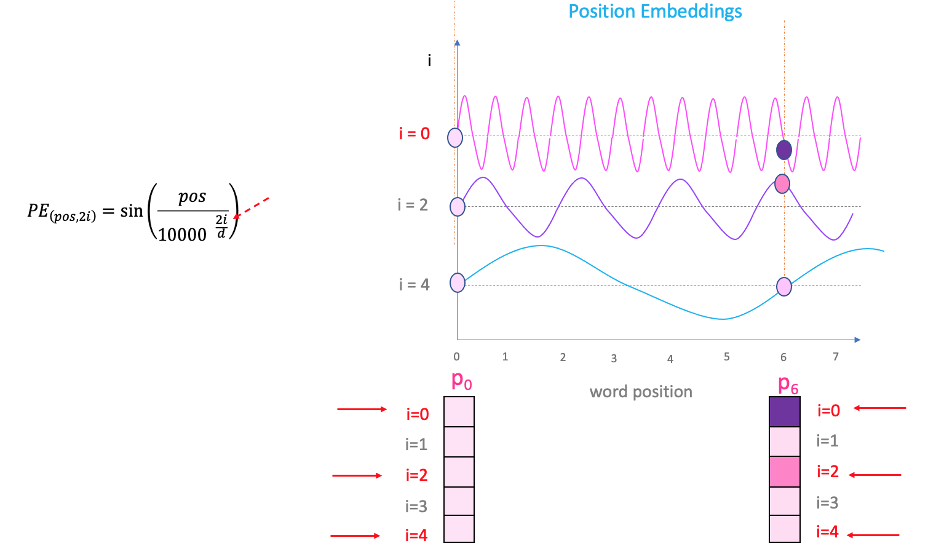
Formula:
\[\begin{align*} PE_{(pos, 2i)} &= \sin\left(\frac{pos}{10000^{2i / d_{\text{model}}}}\right) \\ PE_{(pos, 2i+1)} &= \cos\left(\frac{pos}{10000^{2i / d_{\text{model}}}}\right) \end{align*}\] -
Implementation:
import torch import math def get_sinusoidal_positional_embeddings(num_positions, embedding_dim): pe = torch.zeros(num_positions, embedding_dim) position = torch.arange(0, num_positions).unsqueeze(1).float() div_term = torch.exp(torch.arange(0, embedding_dim, 2).float() * (-math.log(10000.0) / embedding_dim)) pe[:, 0::2] = torch.sin(position * div_term) pe[:, 1::2] = torch.cos(position * div_term) pe = pe.unsqueeze(0) # Shape: (1, num_positions, embedding_dim) return pe - Pros: No additional parameters; can generalize to longer sequences.
- Cons: May not capture complex positional relationships as effectively as learnable embeddings.
3. Relative Positional Encoding
- Description: Encodes relative distances between patches.
- Pros: Captures relative spatial relationships.
- Cons: More complex to implement; may require modifications to attention mechanisms.
4. 2D Positional Encoding
- Description: Extends positional encoding to two dimensions.
-
Implementation:
import torch import math def get_2d_sinusoidal_positional_embeddings(height, width, embedding_dim): pe = torch.zeros(embedding_dim, height, width) y_pos = torch.arange(0, height).unsqueeze(1).float() x_pos = torch.arange(0, width).unsqueeze(0).float() div_term = torch.exp(torch.arange(0, embedding_dim, 2).float() * (-math.log(10000.0) / embedding_dim)) pe[0::2, :, :] = torch.sin(y_pos * div_term).transpose(0, 1).unsqueeze(2) pe[1::2, :, :] = torch.cos(x_pos * div_term).transpose(0, 1).unsqueeze(1) pe = pe.view(embedding_dim, -1).transpose(0, 1).unsqueeze(0) return pe # Shape: (1, num_patches, embedding_dim) - Pros: Captures both height and width positional information.
- Cons: Increased computational complexity.
Reasons for Using Both Sine and Cosine Functions
1. Unique Positional Representation
- Differentiation Across Dimensions: By alternating sine and cosine functions across the embedding dimensions, each position is assigned a unique combination of values.
- Avoid Symmetry: Using both functions prevents the model from mapping different positions to the same embedding, which could happen if only one function were used.
2. Capture Even and Odd Positional Patterns
- Even and Odd Functions: Sine is an odd function $\sin(-x) = -\sin(x)$, while cosine is an even function $\cos(-x) = \cos(x) $.
- Enhanced Expressiveness: Combining both functions allows the model to represent patterns that depend on even or odd positions in the sequence.
3. Facilitate Learning of Relative Positions
- Linear Relationships: The sinusoidal functions enable the model to learn relative positions through linear transformations.
-
Dot Product Property: The dot product between positional encodings of different positions depends on the relative distance between them, aiding the attention mechanism in focusing on relative positions.
For example, consider two positions $pos$ and $pos’$:
\[\text{PE}(pos + k) = \text{Function of } \text{PE}(pos)\]This property allows the model to generalize to sequence lengths not seen during training.
4. Orthogonality and Signal Representation
- Orthogonal Basis Functions: Sine and cosine functions form an orthogonal basis, which is beneficial for representing signals without interference between dimensions.
- Frequency Variation: Different frequencies in the sine and cosine functions help capture both short-term and long-term dependencies.
5. Smoothness and Continuity
- Continuous Functions: Sine and cosine are continuous and differentiable, which aids in gradient-based optimization during training.
- Smooth Encoding Space: The gradual change in values across positions helps the model learn positional relationships smoothly.
Mathematical Insights
Frequency Encoding
- Varying Frequencies: The use of $10000^{2i / d}$ in the denominator ensures that each dimension corresponds to a sinusoid of a different frequency.
- Low to High Frequencies: Lower dimensions capture long-term dependencies (low frequencies), while higher dimensions capture fine-grained positional differences (high frequencies).
Relative Position Computation
- Example: The difference between positional encodings can be used to compute relative positions.
\(\begin{aligned}
\sin(a) - \sin(b) &=2 \cos\left(\frac{a + b}{2}\right) \sin\left(\frac{a - b}{2}\right)\\
\cos(a) - \cos(b) &=-2 \sin\left(\frac{a + b}{2}\right) \sin\left(\frac{a - b}{2}\right)
\end{aligned}\)
These identities help the model infer the relative distance between tokens. —
Practical Benefits
1. No Additional Parameters
- Parameter-Free: The sinusoidal positional encoding is fixed and does not introduce new parameters to the model.
- Reduced Overfitting Risk: Fewer parameters mean less chance of overfitting, especially on smaller datasets.
2. Generalization to Longer Sequences
- Extrapolation: Since the positional encodings are generated using mathematical functions, the model can handle sequences longer than those seen during training.
- Consistency: The encoding method remains consistent regardless of sequence length.
Visualization

Figure: Visualization of sinusoidal positional encodings for different positions and dimensions.
Summary
- Both sine and cosine functions are used in positional embeddings to provide unique and continuous representations of positions in a sequence.
- This combination allows the Transformer model to capture both absolute and relative positional information, which is crucial for tasks that depend on the order of the input data.
- Using both functions enhances the model’s ability to generalize to sequences of different lengths and improves its understanding of positional relationships between tokens.
3. Embedding Layers and Class Token
Image Patch Embedding
Process:
-
Divide Image into Patches: Split the image into non-overlapping patches.
- For a 224x224 image with a patch size of 16x16: $\text{Number of patches} = \left( \frac{224}{16} \right)^2 = 196$
-
Flatten Patches: Each patch is flattened into a 1D vector.
-
Linear Projection: Project each flattened patch into an embedding space.
Code Example:
import torch
import torch.nn as nn

class PatchEmbedding(nn.Module):
    def __init__(self, image_size=224, patch_size=16, embedding_dim=768):
        super(PatchEmbedding, self).__init__()
        self.image_size = image_size
        self.patch_size = patch_size
        self.embedding_dim = embedding_dim
        self.num_patches = (image_size // patch_size) ** 2

        # Conv2d layer to project patches into embedding space
        self.projection = nn.Conv2d(
            in_channels=3,                      # Input channels (RGB)
            out_channels=embedding_dim,         # Output channels (embedding dimension)
            kernel_size=patch_size,             # Patch size
            stride=patch_size                   # Stride equals patch size (non-overlapping patches)
        )

    def forward(self, x):
        """
        x: Input tensor of shape (batch_size, 3, image_size, image_size)
        """
        batch_size = x.shape[0]
        # Apply convolution to get patch embeddings
        x = self.projection(x)  # Shape: (batch_size, embedding_dim, num_patches_sqrt, num_patches_sqrt)
        # Flatten spatial dimensions
        x = x.flatten(2)        # Shape: (batch_size, embedding_dim, num_patches)
        # Transpose to get shape (batch_size, num_patches, embedding_dim)
        x = x.transpose(1, 2)   # Shape: (batch_size, num_patches, embedding_dim)
        return x
Explanation of Tensor Shapes:
- Input
x:(batch_size, 3, image_size, image_size) - After
self.projection(x):(batch_size, embedding_dim, num_patches_sqrt, num_patches_sqrt) - After
x.flatten(2):(batch_size, embedding_dim, num_patches) - After
x.transpose(1, 2):(batch_size, num_patches, embedding_dim)
Class Token and Its Usage
Purpose:
- Global Representation: Serves as a summary of the entire image.
- Classification: The output corresponding to the class token is used for classification tasks.
Implementation:
self.cls_token = nn.Parameter(
    torch.zeros(1, 1, embedding_dim)
)  # Shape: (1, 1, embedding_dim)
Usage in Forward Pass:
def forward(self, x):
    batch_size = x.shape[0]
    # Get patch embeddings
    x = self.patch_embedding(x)  # Shape: (batch_size, num_patches, embedding_dim)
    # Expand class token to batch size
    cls_tokens = self.cls_token.expand(batch_size, -1, -1)  # Shape: (batch_size, 1, embedding_dim)
    # Concatenate class token with patch embeddings
    x = torch.cat((cls_tokens, x), dim=1)  # Shape: (batch_size, num_patches + 1, embedding_dim)
    # Continue with the model...
Why It Is Used:
- Aggregation Point: Interacts with all other tokens via attention, aggregating information.
- Consistent with NLP Models: Mirrors the [CLS] token used in models like BERT.
4. Transformer Blocks in Sequential Order
Now we’ll go through each component in the order they appear in a Vision Transformer.
Input Patches and Embeddings
- Image Input:
(batch_size, 3, image_size, image_size) - Patch Embedding: Convert image to patches and project to embedding space.
- Output:
(batch_size, num_patches, embedding_dim)
- Output:
Adding Positional Encodings
After obtaining patch embeddings, we add positional encodings to incorporate positional information.
Code Example:
# Assuming 'x' is the patch embeddings: (batch_size, num_patches, embedding_dim)
# Add class token
cls_tokens = self.cls_token.expand(batch_size, -1, -1)  # Shape: (batch_size, 1, embedding_dim)
x = torch.cat((cls_tokens, x), dim=1)  # Shape: (batch_size, num_patches + 1, embedding_dim)
# Add positional embeddings
x = x + self.position_embeddings  # Shape: (batch_size, num_patches + 1, embedding_dim)
Transformer Encoder Layers
Each Transformer encoder layer consists of:
- Layer Normalization
- Multi-Head Attention
- Residual Connection
- Layer Normalization
- Feed-Forward Network
- Residual Connection
Layer Normalization
Purpose:
- Stabilizes Training: Normalizes inputs across the features.
- Applied Before Attention and Feed-Forward Layers.
Formula:
\[\text{LayerNorm}(x) = \gamma \left( \frac{x - \mu}{\sigma + \epsilon} \right) + \beta\]- $x$: Input tensor.
- $\mu$: Mean over the last dimension.
- $\sigma$: Standard deviation over the last dimension.
- $\gamma$, $\beta$: Learnable parameters.
- $\epsilon$: Small constant to prevent division by zero.
Implementation:
self.layer_norm1 = nn.LayerNorm(embedding_dim)  # For first LayerNorm
self.layer_norm2 = nn.LayerNorm(embedding_dim)  # For second LayerNorm
Multi-Head Attention
Concept:
- Self-Attention: Each token attends to all other tokens, including itself.
- Multi-Head: Multiple attention heads allow the model to focus on different parts of the sequence.
Single Attention Head
Scaled Dot-Product Attention:
\[\text{Attention}(Q, K, V) = \text{softmax}\left( \frac{Q K^\top}{\sqrt{d_k}} \right) V\]- RQR: Queries matrix
(batch_size, seq_len, head_dim) - RKR: Keys matrix
(batch_size, seq_len, head_dim) - RVR: Values matrix
(batch_size, seq_len, head_dim) - Rd_kR: Dimension of the keys/queries (
head_dim)
Code Example for Single Head:
import torch
import torch.nn as nn
import torch.nn.functional as F

class SingleHeadAttention(nn.Module):
    def __init__(self, embedding_dim):
        super(SingleHeadAttention, self).__init__()
        self.embedding_dim = embedding_dim
        self.query = nn.Linear(embedding_dim, embedding_dim)  # (batch_size, seq_len, embedding_dim)
        self.key = nn.Linear(embedding_dim, embedding_dim)
        self.value = nn.Linear(embedding_dim, embedding_dim)
        self.scaling_factor = embedding_dim ** 0.5

    def forward(self, x):
        """
        x: Input tensor of shape (batch_size, seq_len, embedding_dim)
        """
        Q = self.query(x)  # Shape: (batch_size, seq_len, embedding_dim)
        K = self.key(x)    # Shape: (batch_size, seq_len, embedding_dim)
        V = self.value(x)  # Shape: (batch_size, seq_len, embedding_dim)
        # Compute attention scores
        scores = torch.matmul(Q, K.transpose(-2, -1)) / self.scaling_factor  # (batch_size, seq_len, seq_len)
        # Apply softmax
        attention_weights = F.softmax(scores, dim=-1)  # (batch_size, seq_len, seq_len)
        # Compute weighted sum of values
        out = torch.matmul(attention_weights, V)  # (batch_size, seq_len, embedding_dim)
        return out
Extending to Multi-Head Attention
Concept:
- Multiple Heads: Split the embedding dimension into
num_headssmaller dimensions. - Parallel Attention: Apply attention independently on each head.
- Concatenate: Combine the outputs from all heads.
Code Example for Multi-Head Attention:
class MultiHeadAttention(nn.Module):
    def __init__(self, embedding_dim, num_heads):
        super(MultiHeadAttention, self).__init__()
        assert embedding_dim % num_heads == 0, "Embedding dimension must be divisible by number of heads."
        self.num_heads = num_heads
        self.head_dim = embedding_dim // num_heads  # Dimension per head
        self.embedding_dim = embedding_dim

        # Linear layers for queries, keys, and values
        self.qkv = nn.Linear(embedding_dim, embedding_dim * 3)
        # Output linear layer
        self.fc_out = nn.Linear(embedding_dim, embedding_dim)

    def forward(self, x):
        """
        x: Input tensor of shape (batch_size, seq_len, embedding_dim)
        """
        batch_size, seq_len, _ = x.shape
        # Compute queries, keys, and values
        qkv = self.qkv(x)  # (batch_size, seq_len, 3 * embedding_dim)
        qkv = qkv.reshape(batch_size, seq_len, 3, self.num_heads, self.head_dim)
        qkv = qkv.permute(2, 0, 3, 1, 4)  # (3, batch_size, num_heads, seq_len, head_dim)
        Q, K, V = qkv[0], qkv[1], qkv[2]  # Each: (batch_size, num_heads, seq_len, head_dim)

        # Compute attention scores
        scores = torch.matmul(Q, K.transpose(-2, -1)) / (self.head_dim ** 0.5)  # (batch_size, num_heads, seq_len, seq_len)
        attention_weights = F.softmax(scores, dim=-1)  # (batch_size, num_heads, seq_len, seq_len)

        # Apply attention weights
        out = torch.matmul(attention_weights, V)  # (batch_size, num_heads, seq_len, head_dim)
        # Concatenate heads
        out = out.transpose(1, 2).contiguous().reshape(batch_size, seq_len, self.embedding_dim)  # (batch_size, seq_len, embedding_dim)
        # Final linear layer
        out = self.fc_out(out)  # (batch_size, seq_len, embedding_dim)
        return out
Explanation of Tensor Shapes:
- Input
x:(batch_size, seq_len, embedding_dim) - After
self.qkv(x):(batch_size, seq_len, 3 * embedding_dim) - Reshape for heads:
(batch_size, seq_len, 3, num_heads, head_dim) - Permute to separate Q, K, V:
(3, batch_size, num_heads, seq_len, head_dim) - Q, K, V: Each
(batch_size, num_heads, seq_len, head_dim) - Compute scores:
(batch_size, num_heads, seq_len, seq_len) - Attention weights: Same shape
- Apply attention:
(batch_size, num_heads, seq_len, head_dim) - Concatenate heads:
(batch_size, seq_len, embedding_dim)
Residual Connections
Purpose:
- Ease of Training: Helps in training deep networks by mitigating the vanishing gradient problem.
- Information Flow: Allows information to flow directly across layers.
Implementation:
- After each sub-layer (attention or feed-forward), add the input to the output.
# Assuming 'x' is the input to the sub-layer
# 'sublayer_output' is the output from the sub-layer
x = x + sublayer_output  # Residual connection
Feed-Forward Network
Structure:
- Consists of two linear layers with an activation function (usually GELU) in between.
Code Example:
class FeedForwardNetwork(nn.Module):
    def __init__(self, embedding_dim, hidden_dim):
        super(FeedForwardNetwork, self).__init__()
        self.fc1 = nn.Linear(embedding_dim, hidden_dim)
        self.fc2 = nn.Linear(hidden_dim, embedding_dim)

    def forward(self, x):
        """
        x: Input tensor of shape (batch_size, seq_len, embedding_dim)
        """
        x = self.fc1(x)     # (batch_size, seq_len, hidden_dim)
        x = F.gelu(x)       # (batch_size, seq_len, hidden_dim)
        x = self.fc2(x)     # (batch_size, seq_len, embedding_dim)
        return x
GELU Activation Function
Formula:
$\text{GELU}(x) = x \cdot \Phi(x)$
- $\Phi(x)$: Standard Gaussian cumulative distribution function.
Why GELU is Used:
- Smooth Activation: Provides a smoother activation than ReLU.
- Empirical Performance: Has shown better performance in Transformer models.
5. Complete Transformer Block Code
Now, we’ll combine all the components into a complete Transformer encoder block.
class TransformerEncoderBlock(nn.Module):
    def __init__(self, embedding_dim, num_heads, hidden_dim, dropout_rate=0.1):
        super(TransformerEncoderBlock, self).__init__()
        self.layer_norm1 = nn.LayerNorm(embedding_dim)
        self.multi_head_attention = MultiHeadAttention(embedding_dim, num_heads)
        self.dropout1 = nn.Dropout(dropout_rate)
        self.layer_norm2 = nn.LayerNorm(embedding_dim)
        self.feed_forward = FeedForwardNetwork(embedding_dim, hidden_dim)
        self.dropout2 = nn.Dropout(dropout_rate)

    def forward(self, x):
        """
        x: Input tensor of shape (batch_size, seq_len, embedding_dim)
        """
        # Layer Norm + Multi-Head Attention + Residual Connection
        attn_input = self.layer_norm1(x)  # (batch_size, seq_len, embedding_dim)
        attn_output = self.multi_head_attention(attn_input)  # (batch_size, seq_len, embedding_dim)
        attn_output = self.dropout1(attn_output)
        x = x + attn_output  # Residual connection

        # Layer Norm + Feed-Forward Network + Residual Connection
        ffn_input = self.layer_norm2(x)  # (batch_size, seq_len, embedding_dim)
        ffn_output = self.feed_forward(ffn_input)  # (batch_size, seq_len, embedding_dim)
        ffn_output = self.dropout2(ffn_output)
        x = x + ffn_output  # Residual connection

        return x  # (batch_size, seq_len, embedding_dim)
6. End-to-End Vision Transformer Model
Now we’ll assemble the entire Vision Transformer model, integrating all components.
import torch
import torch.nn as nn
import torch.nn.functional as F

class VisionTransformer(nn.Module):
    def __init__(
        self,
        image_size=224,
        patch_size=16,
        num_classes=1000,
        embedding_dim=768,
        num_heads=12,
        hidden_dim=3072,
        num_layers=12,
        dropout_rate=0.1
    ):
        super(VisionTransformer, self).__init__()
        self.patch_embedding = PatchEmbedding(image_size, patch_size, embedding_dim)
        num_patches = self.patch_embedding.num_patches

        # Class token
        self.cls_token = nn.Parameter(torch.zeros(1, 1, embedding_dim))

        # Positional embeddings
        self.position_embeddings = nn.Parameter(
            torch.zeros(1, num_patches + 1, embedding_dim)
        )

        # Transformer encoder blocks
        self.encoder_layers = nn.ModuleList([
            TransformerEncoderBlock(embedding_dim, num_heads, hidden_dim, dropout_rate)
            for _ in range(num_layers)
        ])

        # Final layer norm
        self.layer_norm = nn.LayerNorm(embedding_dim)

        # Classification head
        self.mlp_head = nn.Sequential(
            nn.Linear(embedding_dim, num_classes)
        )

    def forward(self, x):
        """
        x: Input tensor of shape (batch_size, 3, image_size, image_size)
        """
        batch_size = x.shape[0]
        # Patch embedding
        x = self.patch_embedding(x)  # (batch_size, num_patches, embedding_dim)
        # Class token
        cls_tokens = self.cls_token.expand(batch_size, -1, -1)  # (batch_size, 1, embedding_dim)
        x = torch.cat((cls_tokens, x), dim=1)  # (batch_size, num_patches + 1, embedding_dim)
        # Add positional embeddings
        x = x + self.position_embeddings  # (batch_size, num_patches + 1, embedding_dim)
        # Transformer encoder layers
        for encoder_layer in self.encoder_layers:
            x = encoder_layer(x)  # (batch_size, num_patches + 1, embedding_dim)
        # Final layer norm
        x = self.layer_norm(x)  # (batch_size, num_patches + 1, embedding_dim)
        # Classification head (using class token)
        cls_output = x[:, 0]  # (batch_size, embedding_dim)
        logits = self.mlp_head(cls_output)  # (batch_size, num_classes)
        return logits
7. Classification Example Using Vision Transformers
Let’s provide an end-to-end example of using the Vision Transformer for image classification.
import torch
import torch.nn as nn
import torchvision.transforms as transforms
from PIL import Image

# Define the model
model = VisionTransformer(
    image_size=224,
    patch_size=16,
    num_classes=1000,
    embedding_dim=768,
    num_heads=12,
    hidden_dim=3072,
    num_layers=12,
    dropout_rate=0.1
)

# Define image transformations
transform = transforms.Compose([
    transforms.Resize((224, 224)),
    transforms.ToTensor(),  # Converts to [0,1] range
    transforms.Normalize(mean=[0.485, 0.456, 0.406],  # ImageNet means
                         std=[0.229, 0.224, 0.225])   # ImageNet stds
])

# Load an image
image = Image.open('path_to_image.jpg').convert('RGB')
input_tensor = transform(image).unsqueeze(0)  # (1, 3, 224, 224)

# Forward pass
logits = model(input_tensor)  # (1, num_classes)

# Get predicted class
predicted_class = torch.argmax(logits, dim=-1).item()

print(f'Predicted class: {predicted_class}')
Explanation:
- Model Initialization: Creates an instance of the Vision Transformer model.
- Transformations: Resizes and normalizes the input image.
- Image Loading: Loads an image and converts it to a tensor.
- Forward Pass: Passes the image through the model to get logits.
- Prediction: Retrieves the class with the highest logit.
8. Drawbacks of Attention Modules
Computational Complexity
- Quadratic Complexity: Self-attention scales with $O(N^2)$, where $N$ is the sequence length (number of patches).
- Memory Consumption: The attention matrix consumes significant memory, limiting scalability for high-resolution images.
Inefficiency with Long Sequences
- High-Resolution Images: Larger images result in more patches, increasing computational cost.
- Scalability Issues: Difficult to process large images without significant resource usage.
9. Overcoming Expensive Attention Modules
Axial Transformers
Concept:
- Decompose Attention: Apply attention along individual axes (height and width) instead of across all tokens.
- Reduction in Complexity: Reduces complexity from $O(N^2)$ to $O(N \sqrt{N})$.
Implementation Example:
class AxialAttention(nn.Module):
    def __init__(self, embedding_dim, num_heads, axis):
        super(AxialAttention, self).__init__()
        self.axis = axis  # 'height' or 'width'
        self.embedding_dim = embedding_dim
        self.num_heads = num_heads
        self.multi_head_attention = MultiHeadAttention(embedding_dim, num_heads)

    def forward(self, x):
        """
        x: Input tensor of shape (batch_size, embedding_dim, height, width)
        """
        batch_size, embedding_dim, height, width = x.shape

        if self.axis == 'height':
            # Reshape to apply attention along height
            x = x.permute(0, 3, 2, 1)  # (batch_size, width, height, embedding_dim)
            x = x.reshape(batch_size * width, height, embedding_dim)  # (batch_size * width, height, embedding_dim)
            x = self.multi_head_attention(x)  # (batch_size * width, height, embedding_dim)
            x = x.reshape(batch_size, width, height, embedding_dim).permute(0, 3, 2, 1)  # (batch_size, embedding_dim, height, width)
        elif self.axis == 'width':
            # Reshape to apply attention along width
            x = x.permute(0, 2, 3, 1)  # (batch_size, height, width, embedding_dim)
            x = x.reshape(batch_size * height, width, embedding_dim)  # (batch_size * height, width, embedding_dim)
            x = self.multi_head_attention(x)  # (batch_size * height, width, embedding_dim)
            x = x.reshape(batch_size, height, width, embedding_dim).permute(0, 3, 1, 2)  # (batch_size, embedding_dim, height, width)
        else:
            raise ValueError("Axis must be 'height' or 'width'.")

        return x  # (batch_size, embedding_dim, height, width)
Benefits:
- Efficiency: Reduces computational and memory requirements.
- Scalability: More suitable for high-resolution images.
10. Conclusion
In this comprehensive guide, we’ve explored:
- Vision Transformers: Applying Transformers to vision tasks by treating images as sequences of patches.
- Positional Encoding: Essential for injecting spatial information into the model.
- Embedding Layers and Class Token: How images are converted into sequences of embeddings and the role of the class token.
- Transformer Encoder Blocks: Detailed explanation of each component in the block.
- Complete Model Implementation: Assembling all components into a functional Vision Transformer model.
- Classification Example: Using the model for an image classification task.
- Drawbacks and Solutions: Challenges with attention mechanisms and methods like Axial Transformers to address them.
Key Takeaways:
- Vision Transformers offer a powerful alternative to convolutional neural networks.
- Understanding each component is crucial for implementing and optimizing ViTs.
- Efficient attention mechanisms are important for scaling ViTs to high-resolution images.