Variational Autoencoders (VAEs): A Complete Tutorial

---

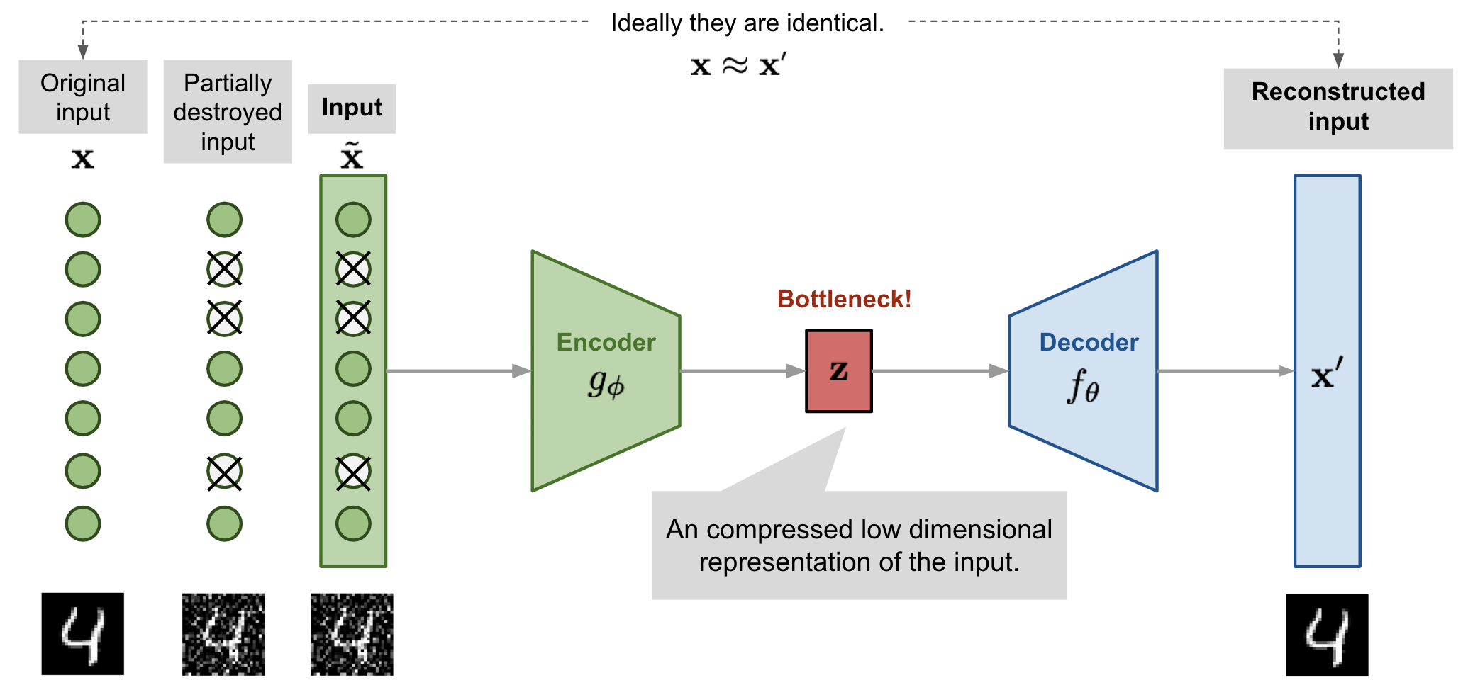
Fig. 1 the structure of variational autoencoder.

🔧 Problem Statement: Why Do We Need VAEs?

We want to learn a generative model that can:

• Sample new data (e.g., images, audio)
• Learn interpretable latent variables
• Model uncertainty in data

We assume the observed data $x$ is generated from a latent variable $z$ using the process:

1. Sample $z \sim p(z)$ from a known prior (e.g., $\mathcal{N}(0, I)$)
2. Sample $x \sim p_\theta(x \mid z)$

This gives the marginal likelihood:

\[(1) \quad p_\theta(x) = \int p_\theta(x \mid z) \cdot p(z) \, dz\]

However, this integral is intractable. To train the model, we need a way to estimate or bound $p_\theta(x)$.

---

❓ Why Not Just Sample from the Prior and Decode?

We can sample $z \sim p(z)$ and decode to $x \sim p_\theta(x \mid z)$. But to train the decoder, we need to:

• Know what $z$ should produce which $x$
• Learn from real $x$’s, which requires recovering a corresponding $z$

But $z$ is unobserved. We don’t know it. To learn the decoder, we must infer $z$ from $x$. That is, we need the posterior $p_\theta(z \mid x)$, which is intractable because:

\[(2) \quad p_\theta(z \mid x) = \frac{p_\theta(x \mid z) p(z)}{p_\theta(x)}\]

And $p_\theta(x)$ involves the same intractable integral from (1).

---

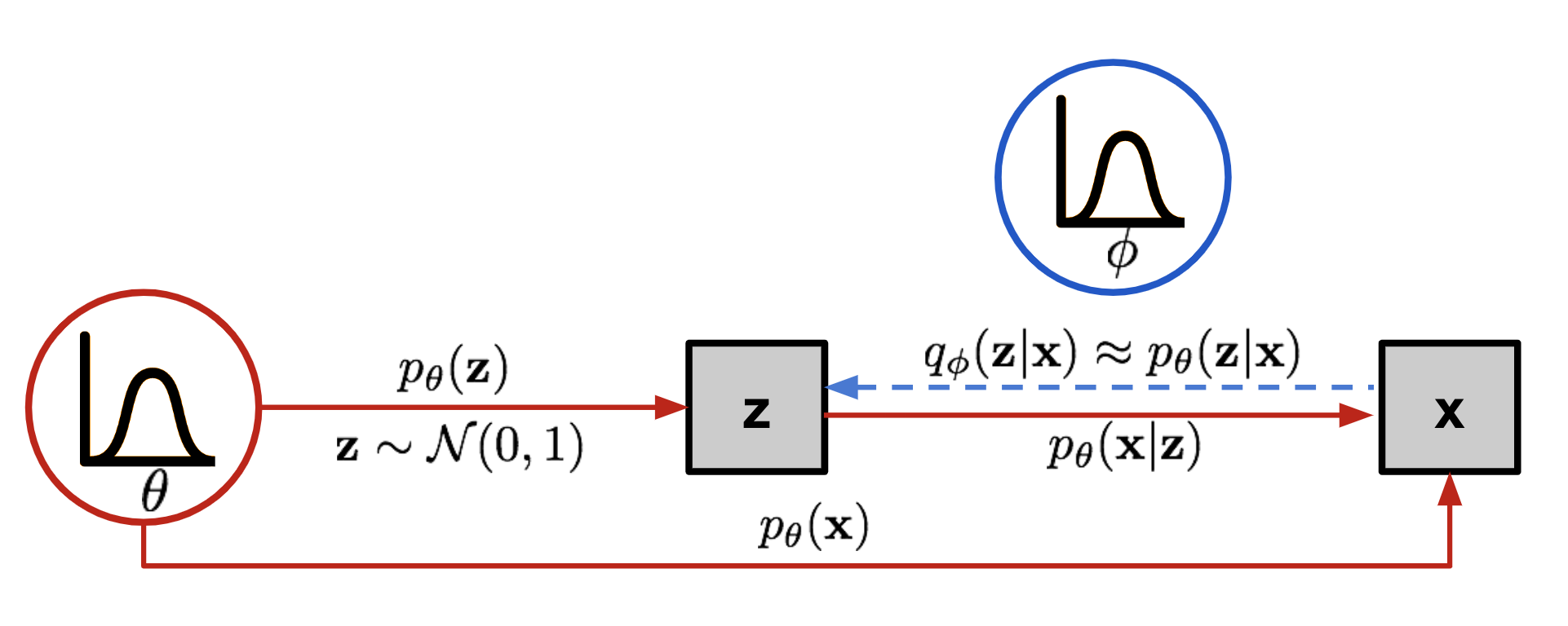
Fig. 2 posterior approximation in vae.

✨ Solution: Approximate the Posterior with an Encoder

We introduce an approximate posterior:

\[(3) \quad q_\phi(z \mid x) \approx p_\theta(z \mid x)\]

This encoder network maps $x$ to a distribution over $z$:

\[(4) \quad q_\phi(z \mid x) = \mathcal{N}(z \mid \mu_\phi(x), \sigma^2_\phi(x) I)\]

Now we can train both:

• Encoder to approximate the posterior
• Decoder to reconstruct $x$ from $z$

---

⚡ Derivation of the ELBO

We want to maximize the data likelihood:

\[(5) \quad \log p_\theta(x) = \log \int p_\theta(x \mid z) p(z) dz\]

Introduce $q_\phi(z \mid x)$ and rewrite:

\[(6) \quad \log p_\theta(x) = \log \int q_\phi(z \mid x) \cdot \frac{p_\theta(x, z)}{q_\phi(z \mid x)} dz\]

Apply Jensen’s inequality:

\[(7) \quad \log p_\theta(x) \geq \mathbb{E}_{q_\phi(z \mid x)} \left[ \log \frac{p_\theta(x, z)}{q_\phi(z \mid x)} \right]\]

This is the Evidence Lower Bound (ELBO):

\[(8) \quad \mathcal{L}(\theta, \phi; x) = \mathbb{E}_{q_\phi(z \mid x)}[\log p_\theta(x \mid z)] - D_{\text{KL}}(q_\phi(z \mid x) \| p(z))\]

• The first term encourages accurate reconstruction
• The second term regularizes $q_\phi(z \mid x)$ to stay close to the prior $p(z)$

---

🌈 Reparameterization Trick

We reparameterize $z$ to allow backpropagation:

\[(9) \quad z = \mu_\phi(x) + \sigma_\phi(x) \cdot \epsilon, \quad \epsilon \sim \mathcal{N}(0, I)\]

This makes $z$ a differentiable function of $x$ and $\epsilon$.

---

🧮 KL Divergence Between Two Gaussians

We compute the KL divergence between the approximate posterior $q(z \mid x) = \mathcal{N}(\mu, \sigma^2)$ and the prior $p(z) = \mathcal{N}(0, 1)$ using the closed-form expression:

\[(10) \quad D_{\text{KL}}(q(z \mid x) \| p(z)) = \frac{1}{2} \sum \left( \mu^2 + \sigma^2 - \log \sigma^2 - 1 \right)\]

Since we often work with $\log \sigma^2$ (denoted logvar), we rewrite:

\[(11) \quad D_{\text{KL}} = -\frac{1}{2} \sum \left( 1 + \log \sigma^2 - \mu^2 - \sigma^2 \right)\]

This gives the exact PyTorch implementation:

kl = -0.5 * torch.sum(1 + logvar - mu.pow(2) - logvar.exp())

• logvar is $\log \sigma^2$
• torch.exp(logvar) gives $\sigma^2$
• mu.pow(2) gives $\mu^2$

This derivation allows efficient and exact KL computation between two diagonal Gaussians. Let me know if you want me to try inserting this again using a different method.

🔢 Summary

Concept	Role
$p(z)$	Prior: fixed $\mathcal{N}(0, I)$
$p_\theta(x \mid z)$	Decoder: likelihood of data given latent
$q_\phi(z \mid x)$	Encoder: approximate posterior
ELBO	Training objective maximizing a lower bound on $\log p(x)$

By maximizing the ELBO, we can jointly train encoder and decoder networks to form a generative model that both reconstructs input data and regularizes its latent space.

---

💡 Example: VAE Training Loop for MNIST (With Defined Encoder and Decoder)

import torch
import torch.nn as nn
import torch.nn.functional as F
from torch.utils.data import DataLoader
from torchvision import datasets, transforms

# Define Encoder: x ➝ μ, logσ²
class Encoder(nn.Module):
    def __init__(self, latent_dim):
        super().__init__()
        self.fc1 = nn.Linear(784, 256)               # (N, 784) ➝ (N, 256)
        self.fc_mu = nn.Linear(256, latent_dim)      # (N, 256) ➝ (N, latent_dim)
        self.fc_logvar = nn.Linear(256, latent_dim)  # (N, 256) ➝ (N, latent_dim)

    def forward(self, x):
        x = x.view(-1, 784)                          # reshape input to (N, 784)
        h = F.relu(self.fc1(x))                      # (N, 784) ➝ (N, 256)
        return self.fc_mu(h), self.fc_logvar(h)      # both: (N, latent_dim)

# Define Decoder: z ➝ x̂
class Decoder(nn.Module):
    def __init__(self, latent_dim):
        super().__init__()
        self.fc1 = nn.Linear(latent_dim, 256)        # (N, latent_dim) ➝ (N, 256)
        self.fc2 = nn.Linear(256, 784)               # (N, 256) ➝ (N, 784)

    def forward(self, z):
        h = F.relu(self.fc1(z))                      # (N, latent_dim) ➝ (N, 256)
        x_hat = torch.sigmoid(self.fc2(h))           # (N, 256) ➝ (N, 784)
        return x_hat.view(-1, 1, 28, 28)              # reshape to (N, 1, 28, 28)

# Reparameterization trick
def reparameterize(mu, logvar):
    std = torch.exp(0.5 * logvar)                    # (N, latent_dim)
    eps = torch.randn_like(std)                     # (N, latent_dim)
    return mu + eps * std                           # (N, latent_dim)

# VAE class combining encoder and decoder
class VAE(nn.Module):
    def __init__(self, latent_dim):
        super().__init__()
        self.encoder = Encoder(latent_dim)
        self.decoder = Decoder(latent_dim)

    def forward(self, x):
        mu, logvar = self.encoder(x)                # ➝ (N, latent_dim) each
        z = reparameterize(mu, logvar)              # ➝ (N, latent_dim)
        x_hat = self.decoder(z)                     # ➝ (N, 1, 28, 28)
        return x_hat, mu, logvar

# Loss function (ELBO)
def loss_fn(x_hat, x, mu, logvar):
    recon = F.binary_cross_entropy(x_hat, x, reduction='sum')
    kl = -0.5 * torch.sum(1 + logvar - mu.pow(2) - logvar.exp())
    return recon + kl

# Data pipeline
transform = transforms.ToTensor()
dataset = datasets.MNIST(root='./data', train=True, download=True, transform=transform)
dataloader = DataLoader(dataset, batch_size=128, shuffle=True)

# Training loop
vae = VAE(latent_dim=20)
optimizer = torch.optim.Adam(vae.parameters(), lr=1e-3)

for epoch in range(10):
    total_loss = 0
    for x, _ in dataloader:
        x_hat, mu, logvar = vae(x)
        loss = loss_fn(x_hat, x, mu, logvar)

        optimizer.zero_grad()
        loss.backward()
        optimizer.step()

        total_loss += loss.item()
    print(f"Epoch {epoch+1}, Loss: {total_loss:.2f}")

This full training loop includes an encoder that maps inputs to a distribution over latent variables, a decoder that reconstructs inputs, and a reparameterization trick to enable gradient flow.