TrackFormer
Below is a comprehensive explanation of TrackFormer, its motivation, architecture, training procedure, inference strategy, and evaluation metrics. The explanation includes conceptual understanding, block diagrams, mathematical details, ground truth generation, loss computation, and pseudo-code snippets with inline comments on tensor shapes. The pseudo-code is illustrative rather than exact.
Intuition and Motivation
Intuition:
Traditional multi-object tracking (MOT) systems often follow a two-step pipeline:
- Detect objects in each frame independently.
- Associate detections across frames to form trajectories.
This separation can lead to suboptimal solutions since detection and association are treated as separate problems. TrackFormer merges these steps by extending a Transformer-based detection architecture (inspired by DETR) to simultaneously detect and track objects. It does this by introducing track queries that carry information about previously tracked objects forward in time, allowing the network to reason about detection and association in a unified end-to-end manner.
Motivation:
- End-to-end training without the need for hand-crafted association heuristics.
- Leveraging Transformers’ ability to handle sets directly, enabling joint reasoning about detection and temporal continuity.
- Improved robustness to occlusions and appearance changes since the model learns both detection and association features together.
Model Overview and Block Diagram
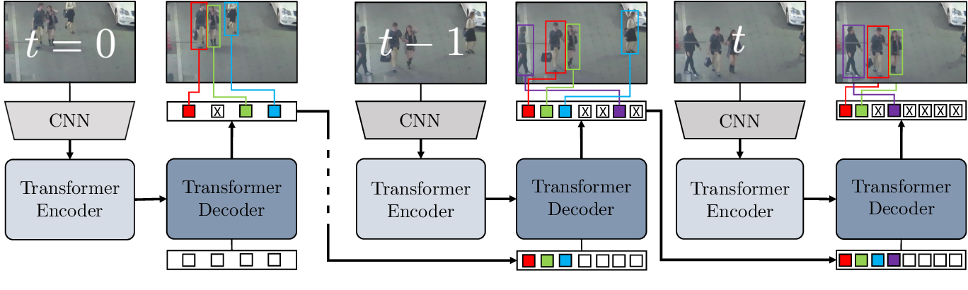
High-Level Architecture: TrackFormer is built upon a Transformer-based object detector (like DETR). The key difference is that it processes a video sequence frame-by-frame and maintains a set of track queries that represent ongoing tracked objects. When a new frame arrives:
- The model extracts image features via a CNN backbone.
- A Transformer encoder processes these features.
- The Transformer decoder receives two sets of queries:
- Detection queries (new object queries): These are learned queries that try to detect new objects in the current frame.
- Track queries (from previous frames): These carry information about previously detected objects, allowing the model to link the same object across frames.
The output is a set of predictions (class labels, boxes, track embeddings) that represent both new detections and updates to existing tracks.
Block Diagram (Conceptual):
      ┌───────────────────────┐
      │       Input Frame     │
      └───┬───────────────────┘
          │ (B,3,H,W)
          v
      ┌───────────────────────┐    ┌─────────────────────────┐
      │       CNN Backbone     │--> │   Positional Encoding    │
      └───┬───────────────────┘    └─────────────────────────┘
          │ (B, C, H', W')
          v
      ┌────────────────────────────────┐
      │   Flatten + Transformer Encoder│
      └───┬────────────────────────────┘
          │ (B, N_enc, D)
          v
     ┌──────────────────────────────────────────┐
     │           Transformer Decoder             │
     │   Inputs: Detection queries + Track queries│
     └───┬──────────────────────────────────────┘
         │ (B, N_query_total, D)
         v
      ┌────────────────────────────────┐
      │     Output Predictions          │
      │  Boxes, Classes, Track Embeds   │
      └────────────────────────────────┘
Where:
- \(B\): Batch size
- \(H,W\): Original image dimensions
- \(H',W'\): Downsampled feature map size
- \(C\): Channels from backbone
- \(D\): Transformer model dimension
- \[N_{enc} = H' \times W'\]
- \[N_{query_{total}} = N_{detect} + N_{track}\]
Mathematics Behind TrackFormer
Feature Extraction:
- CNN backbone: Extracts feature maps \(\mathbf{F} \in \mathbb{R}^{B \times C \times H' \times W'}\).
Positional Encodings:
-
Add 2D sinusoidal positional embeddings to encode spatial positions:
\[\mathbf{E} = \mathbf{F} + \mathbf{P}, \quad \mathbf{E} \in \mathbb{R}^{B \times D \times H' \times W'}\]
Transformer Encoder:
- Flatten \(\mathbf{E}\) to \(\mathbf{E}_{flat} \in \mathbb{R}^{B \times N_{enc} \times D}\).
- Pass through \(L\) encoder layers of self-attention + FFN.
Transformer Decoder:
- Let \(\mathbf{Q}_{detect} \in \mathbb{R}^{B \times N_{detect} \times D}\) be learned detection queries.
- Let \(\mathbf{Q}_{track}^{(t-1)} \in \mathbb{R}^{B \times N_{track} \times D}\) be track queries from the previous frame \(t-1\).
- Concatenate: \(\mathbf{Q}_{total} = [\mathbf{Q}_{detect}; \mathbf{Q}_{track}^{(t-1)}]\)
-
The decoder performs cross-attention with encoder output and self-attention among queries:
\[\mathbf{Q}_{out} \in \mathbb{R}^{B \times (N_{detect}+N_{track}) \times D}\]
Predictions:
- For each query, predict:
- Class distribution \(\hat{p}_i(c)\)
- Bounding box \(\hat{b}_i\)
- Track embedding \(\hat{e}_i\) to identify continuity with previous frames.
Track Update:
- The track queries for the next frame \(\mathbf{Q}_{track}^{(t)}\) are chosen from \(\mathbf{Q}_{out}\) based on assigned matches to previously tracked objects.
Ground Truth Generation
Per Frame Ground Truth:
- Each frame has ground-truth object boxes \(\{b_j\}\) and their IDs (for multi-object tracking).
- The ground-truth includes:
- Class label \(c_j\)
- Box coordinates \(b_j\)
- Track ID \(id_j\)
Correspondence Across Frames:
- The same object ID in consecutive frames forms a track.
- During training, a bipartite matching (Hungarian algorithm) is applied to match predicted boxes to ground-truth boxes, considering both detection and track assignment.
- Ground truth track embeddings are implicit: each object ID should map consistently to the same query across frames.
Loss Function
TrackFormer uses a set-based loss similar to DETR, extended for tracking:
- Hungarian Matching: Find a permutation \(\sigma\) that matches predicted objects to ground-truth objects optimally based on a cost function that includes:
- Classification cost: \(-\log \hat{p}_{\sigma(j)}(c_j)\)
- Box loss: L1 + GIoU loss between \(\hat{b}_{\sigma(j)}\) and \(b_j\)
- Track consistency cost: encourages the model to keep the same query for the same object across frames.
The total loss:
\[\mathcal{L} = \lambda_{class}\mathcal{L}_{class} + \lambda_{box}\mathcal{L}_{box} + \lambda_{track}\mathcal{L}_{track}\]Data Augmentation
Similar to DETR, data augmentation may involve:
- Random resizing, cropping
- Color jittering
- Horizontal flips
- Possibly temporal augmentations like skipping frames or jittering object positions
All augmentations are applied consistently across frames in a sequence.
Training Procedure
- Input Preparation:
- Load a sequence of frames.
- Apply augmentations consistently across all frames.
- Pass each frame through the model and maintain track queries over time.
- Loss Computation:
- For each frame, match predictions to ground truth.
- Compute the detection + tracking loss.
- Backpropagate and update model parameters.
- Iterate Over Epochs:
- Training proceeds over multiple epochs until convergence.
Pseudo-code (PyTorch-like) for Training Loop:
for epoch in range(num_epochs):
    model.train()
    for video_seq in dataloader:
        # video_seq: a batch of video sequences (B, T, 3, H, W)

        # Apply augmentations
        video_seq = augment(video_seq)  # still (B,T,3,H,W)

        track_queries = None  # initialize empty or learned track queries

        total_loss = 0.0
        for t in range(T):
            frame = video_seq[:, t]  # (B, 3, H, W)

            # Forward pass
            outputs, track_queries = model(frame, track_queries)
            # outputs: dict with class_scores(B,N,Dclass), boxes(B,N,4), embeddings(B,N,D)
            # track_queries: updated track queries for next frame (B,Ntrack,D)

            # Get ground truth for this frame
            gt_boxes, gt_classes, gt_ids = get_gt_for_frame(...)
            # gt_boxes: (B,M,4), gt_classes: (B,M), gt_ids: (B,M)

            # Compute Hungarian matching and loss
            loss = compute_loss(outputs, gt_boxes, gt_classes, gt_ids)
            total_loss += loss

        total_loss.backward()
        optimizer.step()
        optimizer.zero_grad()
Inference Procedure
- Initialization:
- For the first frame, only detection queries are used (no tracks yet).
- For Each Subsequent Frame:
- Pass previous track queries and detection queries to the model.
- The model outputs predictions (boxes, classes).
- Use a confidence threshold to decide if a track continues or a new track is started.
- Update the set of track queries based on predictions. Some queries remain for continuous tracks, new queries replace lost/unmatched tracks.
No Hungarian matching is needed at inference; the model directly provides the best association via its track queries.
Pseudo-code for Inference:
model.eval()
track_queries = None

for t in range(T):
    frame = video_seq[:, t]  # (B, 3, H, W)
    outputs, track_queries = model(frame, track_queries)
    # outputs: class scores, boxes, track embeddings
    # track_queries now represent ongoing tracks

    # Filter outputs by confidence
    keep = outputs["class_scores"].max(dim=-1).values > threshold
    final_boxes = outputs["boxes"][keep]
    final_classes = outputs["class_scores"].argmax(dim=-1)[keep]

    # track_queries already updated in model call
    # Associate final boxes with track ids as given by model’s internal track ordering
Metrics
For multi-object tracking, standard metrics include:
- MOTA (Multiple Object Tracking Accuracy): Measures how many objects are missed, falsely detected, or mismatched.
- IDF1 (ID F1-Score): F1-score based on trajectory matching, focusing on identity preservation.
- HOTA (Higher Order Tracking Accuracy): Balances detection and association quality.
- MT (Mostly Tracked), ML (Mostly Lost), FP (False Positives), FN (False Negatives), ID switches.
These metrics evaluate how well the model keeps consistent identities across time, as well as detection quality.
Below is a detailed explanation of common metrics used in multi-object tracking (MOT). We focus on MOTA, IDF1, and HOTA as key metrics, and also describe MT, ML, FP, FN, and ID switches. For each metric, we give its formula (where applicable) and explain the intuition behind it.
Multiple Object Tracking Accuracy (MOTA)
Formula:
\(\text{MOTA} = 1 - \frac{\text{FN} + \text{FP} + \text{IDSW}}{\text{GT}}\)
Where:
- FN: Number of False Negatives (missed detections)
- FP: Number of False Positives (spurious detections)
- IDSW (ID switches): Number of times an object’s identity changes during the track
- GT: Total number of ground truth objects (over all frames)
Intuition:
MOTA is a global measure of how well the tracker performs in terms of detection and identity consistency. It takes into account missed detections, false alarms, and identity switches.
- A high MOTA means fewer misses, fewer false detections, and fewer identity switches.
- If your tracker perfectly detects all objects in all frames without any identity confusion, MOTA would be 1 (or 100%).
IDF1 (ID F1 Score)
Formula:
IDF1 is the F1-score computed over trajectory-level matches. It considers the identity matches over the entire sequence, not just frame by frame. The formula can be written as:
\(\text{IDF1} = \frac{2 \times \text{IDTP}}{2 \times \text{IDTP} + \text{IDFP} + \text{IDFN}}\)
Where:
- IDTP (ID True Positives): The number of detections that correctly match an object’s identity.
- IDFP (ID False Positives): The number of detections that are assigned to the wrong object’s identity.
- IDFN (ID False Negatives): The number of object instances that go undetected or unassigned to the correct identity.
Intuition:
IDF1 focuses on how well the tracker maintains the correct identities over time. Instead of just measuring detection accuracy, IDF1 looks at how many objects are correctly followed with the right ID throughout their lifespan in the sequence.
- A high IDF1 means the tracker rarely loses track of an object’s identity, maintaining a consistent identity match with the ground truth.
Higher Order Tracking Accuracy (HOTA)
Formula (simplified concept):
HOTA decomposes the evaluation into two aspects: detection quality and association quality. It then computes a combined score over a range of thresholds. The main idea is:
\(\text{HOTA} = \frac{1}{|R|} \sum_{r \in R} \sqrt{\text{DetA}(r) \times \text{AssA}(r)}\)
Where:
- \(R\) is a set of recall or IoU thresholds.
- \(\text{DetA}(r)\) (Detection Accuracy) measures how well objects are detected at threshold \(r\).
- \(\text{AssA}(r)\) (Association Accuracy) measures how well tracks are associated across frames at threshold \(r\).
Intuition:
HOTA tries to balance both detection and association performance in a single metric. Unlike MOTA, which mixes errors into one ratio, HOTA looks at detection and association separately and then combines them. By taking the geometric mean of detection and association accuracies, HOTA ensures that both need to be good for a high score.
- A high HOTA means the model is good at detecting objects and maintaining their identities consistently.
Additional Metrics
-
Mostly Tracked (MT):
The percentage of ground-truth objects that are successfully tracked for more than 80% of their lifespan.Intuition:
If an object appears in 50 frames, and the tracker correctly tracks it in at least 40 of these, that object counts as “mostly tracked.” A high MT means the tracker is able to follow most objects for the majority of their existence in the video. -
Mostly Lost (ML):
The percentage of ground-truth objects that are tracked for less than 20% of their lifespan.Intuition:
A high ML means the tracker often loses objects shortly after they appear, failing to maintain track on them. -
False Positives (FP):
The number of detections for non-existent objects (noise detections).Intuition:
FP measures how often the tracker claims an object is present when it is not. A low FP is desired. -
False Negatives (FN):
The number of missed detections of existing objects.Intuition:
FN measures how many times the tracker fails to detect an object that is actually there. A low FN means the tracker rarely misses actual objects. -
ID Switches (IDSW):
The number of times a tracked object’s identity changes from one ID to another during tracking.Intuition:
ID switches measure the stability of the identity assignment. A low IDSW means the tracker consistently assigns the correct ID to the same object over time.
Summary of Intuition
- MOTA: A holistic measure, but it mixes detection and association errors together.
- IDF1: Focuses on identity consistency over entire trajectories.
- HOTA: Balances detection and association into a single metric, ensuring improvement in one area is not overshadowed by poor performance in the other.
- MT, ML, FP, FN, IDSW: Provide granular insight into specific aspects of performance, such as how often objects are mostly tracked, mostly lost, and how frequently false positives/negatives occur, and how stable the identity assignments are.
These metrics together provide a comprehensive view of a tracker’s performance, covering detection quality, identity assignment, and long-term tracking stability.
Summary:
- Intuition & Motivation: Combine detection and tracking in a single end-to-end framework using Transformer queries.
- Architecture: A Transformer encoder-decoder with detection queries and track queries.
- Mathematics: Uses a set-based matching (Hungarian) and transformer attention to produce boxes and track embeddings.
- Ground Truth & Loss: Hungarian matching on each frame for class+box+track continuity.
- Augmentations: Similar to DETR, applied consistently across frames.
- Training: End-to-end with gradients backpropagated through both detection and tracking computations.
- Inference: Sequential frame processing, track queries maintain continuity, no separate association step.
- Metrics: MOTA, IDF1, HOTA for evaluating tracking performance.