Support Vector Machines (SVMs)
1. SVM Analogy: Medical School Admission
Imagine you’re trying to decide whether students get into medical school based on two features:
- GPA (Grade Point Average)
- MCAT score (Medical College Admission Test)
Plotting these as points in 2D space (GPA on x-axis, MCAT on y-axis), suppose accepted students are mostly in the upper-right (high GPA, high MCAT), while rejected students are in the lower-left.
We aim to find a decision boundary (a line) that separates the two classes.
Definitions:
- Hyperplane: In 2D, this is a line. In general, it’s an (n-1)-dimensional flat subspace separating two classes.
- Margin: The distance between the hyperplane and the closest points from each class.
- Support Vectors: The data points that lie exactly on the margin boundaries. These are the critical points that “support” the hyperplane.
- Optimal Hyperplane: The one that maximizes the margin between classes.
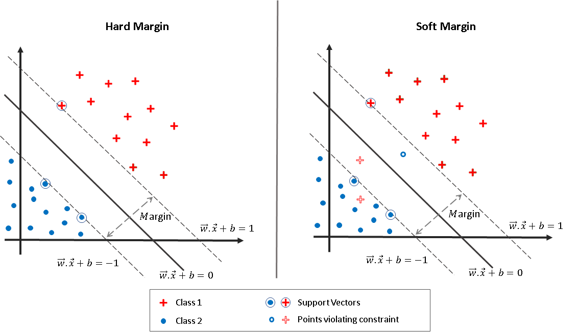
Fig.~1 Support Vector Machines, Hard Marging SVM (left) vs Soft Margin SVM (right) where some outliers are allowed with a penalty
2. Hard Margin SVM (Linearly Separable Case)
We assume the data is perfectly linearly separable.
Goal:
Find a hyperplane $w^T x + b = 0$ that:
- Separates the data.
- Maximizes the margin (i.e., minimizes $|w|^2$).
Formulation:
Let $(x_i, y_i)$ be the training data with $y_i \in {-1, +1}$
Constraints:
\[y_i(w^T x_i + b) \geq 1 \quad \forall i\]Optimization Problem:
\[\min_{w, b} \frac{1}{2} \|w\|^2 \quad \text{subject to} \quad y_i(w^T x_i + b) \geq 1\]This is a convex quadratic optimization problem with linear constraints. We solve it using quadratic programming, not gradient descent.
❗ Why Not Gradient Descent?
Hard-margin SVM uses exact inequality constraints: $y_i(w^T x_i + b) \geq 1$. These are not amenable to standard gradient descent:
- We’d have to use penalty methods to turn constraints into penalties, effectively creating a soft-margin SVM.
- The true hard-margin problem is typically solved via quadratic programming solvers, which handle constraints directly.
Thus, gradient descent is not used for training hard-margin SVMs in practice.
Lagrangian Dual Derivation
We derive the dual form by introducing Lagrange multipliers $\alpha_i \geq 0$ for the constraints.
Primal Lagrangian:
\[\mathcal{L}(w, b, \alpha) = \frac{1}{2} \|w\|^2 - \sum_i \alpha_i [y_i(w^T x_i + b) - 1]\]To find the saddle point, we take partial derivatives and set them to zero:
1. Derivative with respect to $w$:
\[\frac{\partial \mathcal{L}}{\partial w} = w - \sum_i \alpha_i y_i x_i = 0 \Rightarrow w = \sum_i \alpha_i y_i x_i\]2. Derivative with respect to $b$:
\[\frac{\partial \mathcal{L}}{\partial b} = -\sum_i \alpha_i y_i = 0 \Rightarrow \sum_i \alpha_i y_i = 0\]Plug back into the Lagrangian:
\[\mathcal{L}(w, b, \alpha) = \frac{1}{2} \left\|\sum_i \alpha_i y_i x_i \right\|^2 - \sum_i \alpha_i \left[y_i\left(\sum_j \alpha_j y_j x_j^T x_i + b\right) - 1\right]\]Simplify:
- First term becomes: $\frac{1}{2} \sum_{i,j} \alpha_i \alpha_j y_i y_j x_i^T x_j$
- Second term: $-\sum_i \alpha_i y_i \sum_j \alpha_j y_j x_j^T x_i = -\sum_{i,j} \alpha_i \alpha_j y_i y_j x_i^T x_j$
- Third term: $-\sum_i \alpha_i y_i b = 0$ by constraint
- Constant: $+\sum_i \alpha_i$
So the dual becomes:
\[\max_{\alpha} \sum_i \alpha_i - \frac{1}{2} \sum_{i,j} \alpha_i \alpha_j y_i y_j x_i^T x_j\]Subject to:
\[\alpha_i \geq 0, \quad \sum_i \alpha_i y_i = 0\]Why Do We Maximize the Dual? (Intuition)
Perfect — let’s address this precisely.
Why is minimizing the primal problem with constraints equivalent to solving the saddle point problem:
\[\min_{\mathbf{w}, b} \max_{\boldsymbol{\alpha} \geq 0} \mathcal{L}(\mathbf{w}, b, \boldsymbol{\alpha})\]Why does this min-max give the same result as solving the original constrained optimization?
This is guaranteed by the Karush-Kuhn-Tucker (KKT) conditions and strong duality — but let’s derive it intuitively and mathematically.
Original Constrained Problem (Primal Form)
We want to solve:
\[\begin{aligned} \min_{\mathbf{w}, b} \quad & \frac{1}{2} \|\mathbf{w}\|^2 \\ \text{s.t.} \quad & y_i(\mathbf{w}^\top \mathbf{x}_i + b) \geq 1 \quad \forall i \end{aligned}\]These are inequality constraints, so we introduce Lagrange multipliers $\alpha_i \geq 0$.
Define the Lagrangian Function
We build:
\[\mathcal{L}(\mathbf{w}, b, \boldsymbol{\alpha}) = \frac{1}{2} \|\mathbf{w}\|^2 - \sum_{i=1}^N \alpha_i \left[ y_i (\mathbf{w}^\top \mathbf{x}_i + b) - 1 \right]\]This combines:
- The objective $\frac{1}{2} |\mathbf{w}|^2$
- The penalties for constraint violation (through $\alpha_i$)
We now look for the saddle point of $\mathcal{L}$:
\[\min_{\mathbf{w}, b} \max_{\boldsymbol{\alpha} \geq 0} \mathcal{L}(\mathbf{w}, b, \boldsymbol{\alpha})\]This saddle point represents:
- Minimizing over $(\mathbf{w}, b)$: trying to reduce the objective
- Maximizing over $\boldsymbol{\alpha} \geq 0$: trying to enforce the constraints
Here’s the deep intuition:
- If a constraint is violated, the corresponding $\alpha_i$ will grow and push the optimizer to satisfy the constraint.
- If a constraint is satisfied, the corresponding $\alpha_i$ will go to 0 (by complementary slackness).
This min-max structure automatically balances satisfying constraints and optimizing the objective.
This dual view also gives us the flexibility to introduce kernels, because it only depends on dot products $x_i^T x_j$.
**Pseudocode: Hard Margin SVM Training **
\[\begin{aligned} &\textbf{Input:} \ \text{Training data } \{(x_i, y_i)\}, \ y_i \in \{-1, +1\} \\ &\textbf{Output:} \ \text{Weight vector } w \text{ and bias } b \\ &1. \ \text{Formulate primal: minimize } \frac{1}{2} \|w\|^2 \\ &\quad \text{subject to } y_i(w^T x_i + b) \geq 1 \ \forall i \\ &2. \ \text{Form Lagrangian and derive dual:} \\ &\quad L(\alpha) = \sum_i \alpha_i - \frac{1}{2} \sum_{i,j} \alpha_i \alpha_j y_i y_j x_i^T x_j \\ &\quad \text{subject to } \sum_i \alpha_i y_i = 0, \ \alpha_i \geq 0 \\ &3. \ \text{Solve using a QP solver to get } \alpha_i \\ &4. \ \text{Compute } w = \sum_i \alpha_i y_i x_i \\ &\quad \text{Select any support vector } x_k, \text{ then compute } b = y_k - w^T x_k \\ &5. \ \text{Return } w, b \end{aligned}\]Inference After Training Hard-Margin SVM
Once we have trained a hard-margin SVM and obtained:
- The Lagrange multipliers $\alpha_i$
- The weight vector $w$
- The bias term $b$
we can perform classification using the linear decision rule.
Step-by-Step Procedure (No Kernel)
-
Solve the dual optimization problem:
\[\max_{\alpha} \sum_i \alpha_i - \frac{1}{2} \sum_{i,j} \alpha_i \alpha_j y_i y_j x_i^T x_j\]Subject to:
\[\alpha_i \geq 0, \quad \sum_i \alpha_i y_i = 0\] -
Obtain the weight vector:
\[w = \sum_i \alpha_i y_i x_i\]Only the support vectors have $\alpha_i > 0$, so the sum is sparse.
-
Compute the bias $b$: Pick any support vector $x_k$ (i.e., with $\alpha_k > 0$):
\[b = y_k - w^T x_k\] -
Classify a new point $x$:
\[f(x) = w^T x + b, \quad \text{prediction: } \text{sign}(f(x))\]
Pseudocode for Inference (Linear, No Kernel)
\[\begin{aligned} &\textbf{Input: } x, \text{ support vectors } \{x_i, y_i, \alpha_i\}, \text{ bias } b \\ &\textbf{Output: } \text{Predicted label } y \\ &1. \ w \leftarrow \sum_i \alpha_i y_i x_i \\ &2. \ f \leftarrow w^T x + b \\ &3. \ \text{Return } \text{sign}(f) \end{aligned}\]This applies when training is done via solving the dual problem without kernels, using only dot products in the original input space.
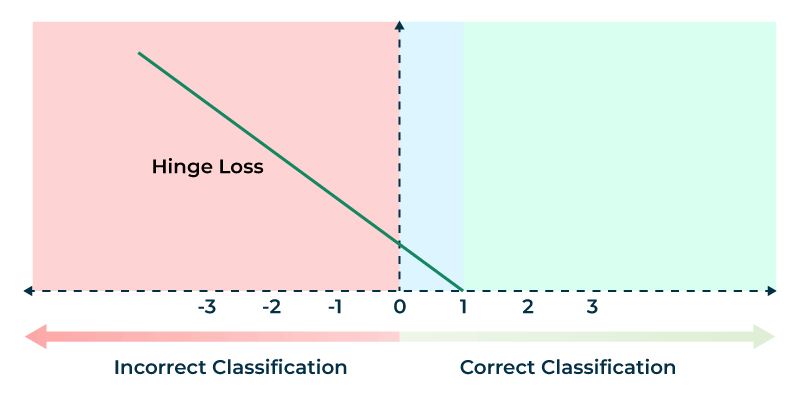
Fig.~2 Hinge loss used in the soft margin SVMs
3. Soft Margin SVM (Handling Non-Separable Data)
In real-world problems (like the med school example), perfect separation is rare. For instance, a student with high GPA and low MCAT might still be accepted, creating an outlier.
To handle such cases, we allow some violations of the margin using slack variables $\xi_i \geq 0$.
Soft Margin SVM Primal Formulation:
We modify the constraints:
\[y_i(w^T x_i + b) \geq 1 - \xi_i\]Objective becomes:
\[\min_{w, b, \xi} \quad \frac{1}{2} \|w\|^2 + C \sum_i \xi_i\]Where:
- $\frac{1}{2} |w|^2$: encourages a large margin
- $\sum \xi_i$: penalizes margin violations
- $C$: trade-off parameter between margin size and violations
Hinge Loss Reformulation
The problem can also be expressed using hinge loss:
\[L(w, b) = \frac{1}{2} \|w\|^2 + C \sum_i \max(0, 1 - y_i(w^T x_i + b))\]- If $y_i(w^T x_i + b) \geq 1$, loss is zero (correctly classified with margin)
- If $y_i(w^T x_i + b) < 1$, we incur linear loss
This form is subdifferentiable and suitable for gradient-based optimization.
Training Soft Margin SVM via Gradient Descent
Let $z_i = y_i(w^T x_i + b)$. Gradient of the hinge loss is: \(\nabla_w L = w - C \sum_{i: z_i < 1} y_i x_i\) \(\nabla_b L = -C \sum_{i: z_i < 1} y_i\)
Pseudocode: Soft Margin SVM (Gradient Descent)
\[\begin{aligned} &\textbf{Input:} \ \text{Training data } \{(x_i, y_i)\}, \text{learning rate } \eta, \text{regularization } C, \text{epochs } T \\ &\textbf{Output:} \ w, b \\ &1. \ \text{Initialize } w = 0, \ b = 0 \\ &2. \ \text{For } t = 1 \text{ to } T:\\ &\quad \text{For each } (x_i, y_i):\\ &\quad\quad \text{Compute margin: } m = y_i(w^T x_i + b) \\ &\quad\quad \text{If } m \geq 1:\\ &\quad\quad\quad w \leftarrow w - \eta w \\ &\quad\quad\quad b \leftarrow b \\ &\quad\quad \text{Else:}\\ &\quad\quad\quad w \leftarrow w - \eta (w - C y_i x_i) \\ &\quad\quad\quad b \leftarrow b + \eta C y_i \\ &3. \ \text{Return } w, b \end{aligned}\]How the Dual Helps in High Dimensions
The dual formulation of SVM is particularly powerful in high-dimensional spaces.
Why?
- In the dual, the data appears only in terms of dot products: $x_i^T x_j$.
- These dot products can be computed without explicitly constructing high-dimensional features via the kernel trick.
- This allows us to work in infinite-dimensional feature spaces (like with the RBF kernel) while computing everything efficiently in the original space.
Intuition:
Even if the data is not linearly separable in its original space, it may be separable in a higher-dimensional space. Instead of transforming all data points manually, we implicitly map them using a kernel, which computes dot products in that higher-dimensional space without ever forming the mapped vectors.
This makes the dual SVM especially suited for high-dimensional or nonlinearly separable problems.
Dual Optimization vs Support Vectors
- The dual optimization problem introduces one Lagrange multiplier $\alpha_i$ for every training point.
- So during training, the dual is optimized over all data points.
- However, after training, most $\alpha_i$ are zero.
- Only the support vectors — points that lie exactly on the margin or violate it — have non-zero $\alpha_i$.
Therefore:
- Dual training involves all data.
- Inference (prediction) only uses support vectors:
This sparsity is a key reason why SVMs are efficient at prediction time.
Kernel Trick: Making SVMs Nonlinear
Why Do We Need Kernels? (Intuition)
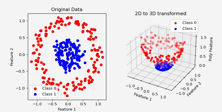
Fig.3 Mapping the features to a new space via a nonlinear transformation does the trick and helps the SVM to linearly separate the data using a hyperplane.
Suppose you have a dataset where class 0 lies in a small circle centered at the origin, and class 1 surrounds it in a ring. Clearly, no straight line (or hyperplane) can separate them in 2D space — the problem is nonlinear.
One idea: manually project the data into a higher-dimensional space. For example, we can map:
\[\phi(x_i) = ((x_i^1)^2, (x_i^2)^2, \sqrt{2}x_i^1x_i^2, \sqrt{2}x_i^1, \sqrt{2}x_i^2, 1)\]This maps the 2D input into a 6-dimensional space where the inner and outer circles can be linearly separated.
To perform classification with a linear SVM in this new space, we need dot products between projected vectors. Let two input vectors be:
\[x_i = (x_i^1, x_i^2), \quad x_j = (x_j^1, x_j^2)\]Then:
\[\phi(x_i)^T \phi(x_j) = (x_i^1)^2(x_j^1)^2 + (x_i^2)^2(x_j^2)^2 + 2x_i^1x_i^2x_j^1x_j^2 + 2x_i^1x_j^1 + 2x_i^2x_j^2 + 1\]But this is exactly:
\[(x_i^T x_j + 1)^2\]This shows that a simple kernel function:
\[K(x_i, x_j) = (x_i^T x_j + 1)^2\]computes the dot product in the 6D feature space without ever computing $\phi(x_i)$ explicitly.
Problems with Manual Feature Mapping
- Requires clever and problem-specific design.
- Explicitly computing $\phi(x_i)$ for all data points becomes infeasible as dimensionality increases.
- Storage and computation cost grow rapidly.
How Kernels Help
The kernel trick allows us to skip computing the high-dimensional mapping $\phi(x_i)$ altogether. Instead of projecting to feature space and doing the dot product, we use:
\[K(x_i, x_j) = \phi(x_i)^T \phi(x_j)\]This allows us to work implicitly in high-dimensional or infinite-dimensional spaces using only functions of dot products in the original space.
This leads to significant savings in computation and memory, especially in large or complex datasets.
Common Kernel Functions
1. Polynomial Kernel
Defined as:
\[K(x_i, x_j) = (x_i^T x_j + c)^d\]- $d$: degree of the polynomial
- $c$: constant to control the influence of higher-order terms
Example (quadratic):
\[K(x_i, x_j) = (x_i^T x_j + 1)^2\]This implicitly maps inputs to a space that includes all degree-2 combinations of features:
\[(x_i^1, x_i^2) \mapsto ((x_i^1)^2, (x_i^2)^2, x_i^1 x_i^2, x_i^1, x_i^2, 1)\]2. Radial Basis Function (RBF) Kernel / Gaussian Kernel
Defined as:
\[K(x_i, x_j) = \exp\left(-\frac{\|x_i - x_j\|^2}{2\sigma^2}\right)\]- $\sigma$: width of the Gaussian
This measures similarity: close points give high values $\approx 1$, distant points yield values $\approx 0$. It corresponds to mapping inputs into an infinite-dimensional space of Gaussian basis functions.
Kernelized Dual Optimization Problem
After applying a kernel, the dual becomes:
\[\max_{\alpha} \sum_i \alpha_i - \frac{1}{2} \sum_{i,j} \alpha_i \alpha_j y_i y_j K(x_i, x_j)\]Subject to:
\[\alpha_i \geq 0, \quad \sum_i \alpha_i y_i = 0\]The prediction function for a new sample $x$ becomes:
\[f(x) = \sum_{i \in \text{SV}} \alpha_i y_i K(x_i, x) + b\]This enables nonlinear separation using a linear classifier in a transformed space.
RBF as Infinite Polynomial Expansion
The standard RBF kernel is defined as:
\[K(x_i, x_j) = \exp\left(-\frac{\|x_i - x_j\|^2}{2\sigma^2}\right)\]We can rewrite the squared norm using the identity:
\[\|x_i - x_j\|^2 = \|x_i\|^2 + \|x_j\|^2 - 2 x_i^T x_j\]So:
\[K(x_i, x_j) = \exp\left(-\frac{\|x_i\|^2}{2\sigma^2}\right) \cdot \exp\left(-\frac{\|x_j\|^2}{2\sigma^2}\right) \cdot \exp\left(\frac{x_i^T x_j}{\sigma^2}\right)\]Let:
\[C(x_i, x_j) = \exp\left(-\frac{\|x_i\|^2 + \|x_j\|^2}{2\sigma^2}\right)\]Then:
\[K(x_i, x_j) = C(x_i, x_j) \cdot \exp\left(\frac{x_i^T x_j}{\sigma^2}\right)\]Now, for any constant $\gamma = 1/\sigma^2$, consider:
\[\exp\left(\gamma x_i^T x_j\right) = \exp\left(\gamma (x_i^T x_j + 1 - 1)\right) = e^{-\gamma} \cdot \exp\left(\gamma (1 + x_i^T x_j)\right)\]So we can write:
\[K(x_i, x_j) = C'(x_i, x_j) \cdot \exp\left(\gamma (1 + x_i^T x_j)\right)\]where $C’(x_i, x_j) = C(x_i, x_j) e^{-\gamma}$.
Finally, apply the Taylor expansion:
\[\exp(\gamma (1 + x_i^T x_j)) = \sum_{n=0}^\infty \frac{\gamma^n}{n!}(1 + x_i^T x_j)^n\]So the full kernel becomes:
\[K(x_i, x_j) = C'(x_i, x_j) \cdot \sum_{n=0}^\infty \frac{\gamma^n}{n!}(1 + x_i^T x_j)^n\]This shows that the RBF kernel is equivalent to a weighted infinite sum of polynomial kernels of the form $(1 + x_i^T x_j)^n$.
Intuition: This expansion reveals how the RBF kernel implicitly combines all polynomial degrees simultaneously, allowing the model to separate data with arbitrarily complex decision boundaries in a smooth and efficient manner — without explicitly computing high-dimensional feature maps.
How the Data Looks in Infinite Polynomial Space
When you transform data using all polynomial functions of all degrees (as the RBF kernel effectively does), you’re projecting each data point into an infinite-dimensional space. Each new dimension corresponds to a different nonlinear combination of the original features:
- degree-1 features: $x_i^1, x_i^2, \ldots$
- degree-2 features: $(x_i^1)^2, x_i^1 x_i^2, \ldots$
- degree-3 features: $(x_i^1)^3, (x_i^1)^2 x_i^2, \ldots$
- … up to infinity
So every data point becomes a vector with infinitely many components, encoding all possible polynomial interactions. In this space:
- Data that was nonlinearly separable in the original space becomes linearly separable because the higher-order dimensions stretch the space so that even complex curved boundaries become flat (linear hyperplanes).
- This is particularly helpful for highly entangled classes or structured patterns (e.g., concentric circles, spirals, etc.).
How SVM Can Handle It
- SVM in its dual form does not require explicitly computing this infinite-dimensional vector.
- It only requires computing dot products in this space — which the RBF kernel does implicitly.
Thus, even though we are conceptually working in infinite dimensions, the kernel trick allows SVM to:
- Represent and compute everything efficiently using only the kernel function.
- Learn a separating hyperplane in this infinite space, which corresponds to a nonlinear decision boundary in the original space.
This is the core power of kernelized SVMs: they transform impossible classification tasks into easy linear separations, all while remaining computationally tractable.
Multiclass SVM: Linear and Nonlinear Cases
SVM is inherently a binary classifier, but it can be extended to multiclass problems using two primary strategies:
1. One-vs-Rest (OvR) Strategy
- For $K$ classes, train $K$ binary SVM classifiers.
- Each classifier $f_k(x)$ learns to distinguish class $k$ vs. all other classes.
-
During inference, evaluate all $f_k(x)$ and pick the class with the highest score:
\[\hat{y} = \arg\max_k f_k(x)\]
2. One-vs-One (OvO) Strategy
- Train $\frac{K(K-1)}{2}$ binary SVM classifiers, each distinguishing a pair of classes.
- During inference, each classifier votes, and the class with the majority of votes is selected.
Linear vs Nonlinear SVM in Multiclass
- Linear Multiclass SVM: Uses linear decision boundaries in original feature space. Suitable for data that is linearly separable or close to it.
- Nonlinear Multiclass SVM: Uses kernels (e.g., polynomial, RBF) to create nonlinear decision boundaries in the input space. Particularly useful for complex, overlapping class structures.
Kernel Multiclass SVM (Nonlinear)
- OvR and OvO strategies still apply.
- Each classifier uses the kernel trick to implicitly operate in high-dimensional space.
- Example: Use RBF kernel in OvR setup to create one nonlinear boundary for each class.
Note: Modern libraries like scikit-learn handle multiclass SVMs automatically using OvR by default. They abstract the training of multiple binary classifiers behind a unified multiclass interface.
Support Vector Regression (SVR)
Support Vector Machines can also be adapted for regression tasks. This version is called Support Vector Regression (SVR).
Key Idea
Instead of finding a hyperplane that separates classes, SVR finds a function that:
- Has at most $\varepsilon$ deviation from the true target values for all training points.
- Is as flat as possible (minimizing $|w|^2$).
Loss Function (ε-insensitive)
SVR introduces the $\varepsilon$-insensitive loss:
\[L_\varepsilon(y, f(x)) = \max(0, |y - f(x)| - \varepsilon)\]This means we ignore errors smaller than $\varepsilon$, and penalize errors beyond it linearly.
Optimization Objective
Minimize:
\[\frac{1}{2}\|w\|^2 + C \sum_{i=1}^n (\xi_i + \xi_i^*)\]Subject to:
\[\begin{cases} y_i - w^T x_i - b \leq \varepsilon + \xi_i \\ w^T x_i + b - y_i \leq \varepsilon + \xi_i^* \\ \xi_i, \xi_i^* \geq 0 \end{cases}\]Here:
- $\xi_i, \xi_i^*$ are slack variables for deviations beyond $\varepsilon$
- $C$ controls the trade-off between flatness and tolerance to errors
Kernelized SVR (Nonlinear Regression)
SVR can also use kernel functions to model nonlinear regression:
\[f(x) = \sum_i (\alpha_i - \alpha_i^*) K(x_i, x) + b\]This is similar to classification SVMs, except the coefficients $\alpha_i, \alpha_i^*$ arise from a different dual problem adapted for regression.
Use Cases
- Forecasting (e.g., stock prices, weather)
- Signal denoising
- Function approximation
SVR offers a robust, margin-based approach to regression with strong generalization ability — especially when used with kernels for nonlinear trends.