A Deep Dive into Speculative Decoding: The Complete Guide

Even with highly optimized systems, the process of generating text from Large Language Models (LLMs) faces a final, stubborn bottleneck: sequential decoding. Generating one token requires a full, time-consuming forward pass through the model. Because this must be done one token at a time, the overall speed is limited by memory latency.

Speculative Decoding is a state-of-the-art inference algorithm that brilliantly overcomes this barrier. It allows a large language model to effectively generate multiple tokens for the cost of a single forward pass, dramatically reducing latency without any loss in output quality.

1. The Core Intuition: The “Intern and Senior Partner” Analogy

To build a strong mental model, imagine a high-stakes law firm.

• The Target LLM ($M_t$) is the “Senior Partner” 👩‍⚖️: A world-class, extremely knowledgeable, and highly accurate lawyer. Their time is valuable, and a consultation (a forward pass) is slow. They are always right.
• The Draft Model ($M_d$) is the “Junior Intern” 👨‍🎓: A fast, eager intern who is much cheaper to consult (a smaller model with lower latency) but might make occasional mistakes.

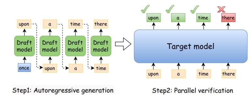
Fig.1 Speculative decoding architecture, the draft model generates the completion token by token and the target model does a one-shot parallel prediction for all the tokens.

The Process:

1. Drafting: Instead of waiting for the partner, you give the current document to the Intern, who quickly writes a draft of the next K words.
2. Parallel Verification: You give this K-word draft to the Senior Partner all at once. Because they can read the full draft in parallel (like a Transformer processing a sequence), they verify it in a single, slow consultation.
3. Acceptance & Correction: You compare the intern’s draft to what the partner would have written. You accept all words that match up until the first mistake. At that point, you take the partner’s single corrected word and discard the rest of the intern’s draft.

The Result: In one “billing cycle” of the expensive Senior Partner, you might get several words approved instead of just one, massively accelerating the process.

2. Key Components and Setup

The Models and Their Outputs

Speculative decoding requires two models that share the same tokenizer.

1. Target Model ($M_t$): The large, high-quality model whose output we want.
2. Draft Model ($M_d$): A much smaller, faster version of the same model.

Both models end with an LM Head, a linear layer that projects the final hidden state $h \in \mathbb{R}^{d_{model}}$ to a vector of raw scores called logits ($z \in \mathbb{R}^{V}$), where V is the vocabulary size. These logits are converted into a probability distribution via the softmax function:

\[p_j = P(\text{token}_j | \text{context}) = \text{softmax}(z)_j = \frac{\exp(z_j)}{\sum_{i=1}^{V} \exp(z_i)}\]

We will denote the target model’s distribution as $q(x)$ and the draft model’s as $p(x)$.

Choosing K: The Number of Draft Tokens

K is the number of tokens the draft model will generate. It’s a hyperparameter with a key trade-off:

• Small K (e.g., 2-3): Low risk of an incorrect draft, but lower potential speedup.
• Large K (e.g., 8-10): High potential for speedup, but a higher risk of an early mismatch, which wastes computation.

In practice, K is often chosen in the range of 4 to 8 to balance this risk and reward.

3. The Algorithm: A Detailed Walkthrough

The algorithm proceeds in a loop. Let the current confirmed sequence of tokens be context.

Phase 1: Drafting Phase

The fast Draft Model ($M_d$) generates K tokens autoregressively. At each step i, it takes the current context, produces a probability distribution $p_i$, and samples a token $x’_i$ (typically via greedy sampling, argmax). This produces a draft sequence $X’ = [x’_1, \dots, x’_K]$ and the corresponding distributions $[p_1, \dots, p_K]$.

Phase 2: Parallel Verification Phase

The Target Model ($M_t$) processes the full sequence context + X' in a single parallel forward pass. This single pass yields K+1 output probability distributions from the target model, which we can represent as a tensor of shape (K+1, V). Let’s call this list of distributions $Q = [q_1, q_2, \dots, q_K, q_{K+1}]$.

Phase 3: Left-to-Right Acceptance & Rejection

This is the core of the algorithm. We iterate from i = 1 to K and decide whether to accept or reject each draft token $x’_i$ using Modified Rejection Sampling.

For each position i, we look at the draft token $x’_i$ and the two distributions for that position, $p_i$ and $q_i$.

1. Calculate Acceptance Probability ($\alpha_i$): We compute the ratio of probabilities assigned to the drafted token by both models.

   \[\alpha_i = \min\left(1, \frac{q_i(x'_i)}{p_i(x'_i)}\right)\]

2. Perform Probabilistic Check: We accept the token $x’_i$ with probability $\alpha_i$. This is done by drawing a random number $r$ from a uniform distribution between 0 and 1.

   • If $r < \alpha_i$, the token is accepted. We continue to the next token.
   • If $r \ge \alpha_i$, the token is rejected. The loop terminates immediately.

The reason for this probabilistic check (instead of a simple threshold) is that it is the standard, unbiased method to realize a decision with a specific probability. It is the core of the rejection sampling technique that mathematically guarantees the final output is statistically identical to the target model’s.

Phase 4: Handling the Sequence: Replacement and Bonus Tokens

The loop through the draft tokens can end in two ways:

1. A Mismatch Occurs (Rejection): Let’s say the check fails at token $i$. All previous $i-1$ tokens have been accepted. The algorithm must stop here because all subsequent target distributions ($q_{i+1}, q_{i+2}, \dots$) were conditioned on the draft token $x’_i$ being correct. Since it was rejected, they are now invalid.
   • The Replacement Token: Instead of just restarting, we use the valid distribution $q_i$ that we already computed. However, we cannot simply sample from $q_i$, as this would bias the output. We must sample from a corrected distribution that accounts for the information gained during rejection.
   • Mathematics of Correction: The new distribution $p’_i$ is formed by taking the “leftover” probability mass where the target model was more confident than the draft model.

\[p'_i(x) = \text{Normalize}\left(\max(0, q_i(x) - p_i(x))\right)\]

• We perform one sample from this distribution $p^\prime_i$ to get a single replacement token, $x_{new}$.

• Cycle Output: The new tokens generated in this cycle are [accepted_tokens] + [x_new].

1. The Entire Draft is Accepted (The Bonus Token): If the loop completes and all K draft tokens are accepted, we get a “bonus.” The target model’s forward pass also computed the distribution for the next token, $q_{K+1}$. We can perform one final sample from this distribution to get a $(K+1)-th$ token for free, maximizing the output from a single target model call.

4. Performance Analysis: Acceptance Rate and Speedup

• Acceptance Rate ($r$): The average probability that any given drafted token will be accepted. It can be proven that this rate is directly related to how similar the draft and target distributions are:

  \[r = \sum_{x \in V} \min(p(x), q(x)) = 1 - \frac{1}{2} \|q - p\|_1\]

  A better draft model leads to a higher acceptance rate.

• Rejection Rate: The probability of rejection is simply $1-r = \frac{1}{2} |q - p|_1$.

• Speedup: The practical speedup is approximately equal to the average number of tokens accepted per cycle, $n_{accepted}$.

  \[\text{Speedup} \approx n_{accepted}\]

  If, on average, 3 tokens are accepted per cycle, you achieve a nearly 3x speedup in wall-clock latency. The small overhead from the draft model is usually negligible.

5. Code Pseudocode

This pseudocode illustrates the full logic.

def speculative_decoding_step(context, target_model, draft_model, K):
    # 1. DRAFTING PHASE: Generate K tokens from the draft model
    draft_tokens, draft_distributions = [], []
    temp_context = context.copy()
    for _ in range(K):
        q_dist = draft_model.get_distribution(temp_context)
        draft_token = torch.argmax(q_dist) # Greedy sample for draft
        draft_tokens.append(draft_token)
        draft_distributions.append(q_dist)
        temp_context.append(draft_token)

    # 2. VERIFICATION PHASE: Get K+1 distributions from the target model
    verification_input = context + draft_tokens
    target_distributions = target_model.get_distributions(verification_input)

    # 3. ACCEPTANCE / REJECTION PHASE
    n_accepted = 0
    for i in range(K):
        p_i = draft_distributions[i]
        q_i = target_distributions[i]
        x_draft_i = draft_tokens[i]

        p_prob = p_i[x_draft_i]
        q_prob = q_i[x_draft_i]

        acceptance_prob = min(1.0, q_prob / p_prob)
        
        if torch.rand(()) < acceptance_prob:
            # Accept the token
            n_accepted += 1
        else:
            # Reject and correct from the (q-p)+ distribution
            p_corrected_dist = F.relu(q_i - p_i) # max(0, q-p)
            p_corrected_dist /= p_corrected_dist.sum() # Normalize
            
            replacement_token = torch.multinomial(p_corrected_dist, 1)
            
            # Return accepted prefix + one corrected token
            return draft_tokens[:n_accepted] + [replacement_token]

    # If all K tokens were accepted, sample the bonus token
    bonus_token_dist = target_distributions[K]
    bonus_token = torch.multinomial(bonus_token_dist, 1)

    return draft_tokens + [bonus_token]

6. Key References

• Modern Formulation: Leviathan, Y., Kalman, M., & Matias, Y., et al. (2022). Fast Inference from Transformers via Speculative Decoding. arXiv preprint arXiv:2211.17192.
• Independent Work & Sampling Variants: Chen, X., Wong, S., & remedial, Z., et al. (2023). Accelerating Large Language Model Decoding with Speculative Sampling. arXiv preprint arXiv:2302.01318.