Kernel-Based Attention and the Performer: Full Tutorial

Performers are Transformer architectures which can estimate regular (softmax) full-rank-attention Transformers with provable accuracy, but using only linear (as opposed to quadratic) space and time complexity, without relying on any priors such as sparsity or low-rankness. To approximate softmax attentionkernels, Performers use a novel Fast Attention Via positive Orthogonal Random features approach (FAVOR+), which may be of independent interest for scalable kernel methods. FAVOR+ can also be used to efficiently model kernelizable attention mechanisms beyond softmax. This representational power is crucial to accurately compare softmax with other kernels for the first time on large-scale tasks, beyond the reach of regular Transformers, and investigate optimal attention-kernels. Performers are linear architectures fully compatible with regular Transformers and with strong theoretical guarantees: unbiased or nearly-unbiased estimation of the attention matrix, uniform convergence and low estimation variance. We tested Performers on a rich set of tasks stretching from pixel-prediction through text models to protein sequence modeling. Performer demonstrates competitive results with other examined efficient sparse and dense attention methods, showcasing effectiveness of the novel attention-learning paradigm leveraged by Performers.

1. What Is a Kernel?

A kernel is a function that computes similarity between two inputs in a possibly high- or infinite-dimensional space without explicitly transforming the data. Formally:

\[k(x, x') = \langle \phi(x), \phi(x') \rangle_\mathcal{H}\]

where:

$\phi: \mathbb{R}^d \rightarrow \mathcal{H}$ is a feature map,
$\mathcal{H}$ is a (possibly infinite) Hilbert space,
$\langle \cdot, \cdot \rangle$ is the inner product in $\mathcal{H}$.

Examples of Kernels and Their Feature Maps

Kernel Name	Formula	Feature Map $\phi(x)$	Dimensionality
Linear	$x^\top x’$	$x$	$d$
Polynomial (deg=d)	$(x^\top x’ + c)^d$	Monomials of degree $\leq d$	$O(d^p)$
Cosine	$\frac{x^\top x’}{\|x\|\|x’\|}$	$\frac{x}{\|x\|}$	$d$
RBF (Gaussian)	$\exp(-\frac{\|x - x’\|^2}{2\sigma^2})$	Infinite-dimensional	$\infty$

2. Random Fourier Features (RFF)

For shift-invariant kernels $k(x - x’)$, Bochner’s theorem tells us:

A continuous, shift-invariant, positive-definite kernel is the Fourier transform of a non-negative probability distribution.

So:

\[k(x, x') = \int e^{i\omega^\top(x - x')} p(\omega) \, d\omega = \mathbb{E}_{\omega \sim p(\omega)}[e^{i\omega^\top x} e^{-i\omega^\top x'}]\]

Using Euler’s formula:

\[e^{i\theta} = \cos \theta + i \sin \theta\]

So:

\[k(x, x') = \mathbb{E}_\omega[\cos(\omega^\top x - \omega^\top x')] = \mathbb{E}_\omega\cos(\omega^\top x) \cos(\omega^\top x') + \sin(\omega^\top x) \sin(\omega^\top x')]\]

Using Monte Carlo approximation we have

\[k(x, x') = \frac1{D}\sum_j\cos(\omega_j^\top x - \omega_j^\top x') = \frac1{D}\sum_j\cos(\omega_j^\top x) \cos(\omega_j^\top x') + \sin(\omega_j^\top x) \sin(\omega_j^\top x')]\]

Defining $\phi_\omega(x)$ we have

\[\phi_\omega(x) = \begin{bmatrix} \cos(\omega^\top x) \\ \sin(\omega^\top x) \end{bmatrix} \Rightarrow k(x, x') \approx \frac{1}{D} \sum_{j=1}^D \phi_{\omega_j}(x)^\top \phi_{\omega_j}(x')\]

with explicit features

\[\phi(x) = \sqrt{\frac{1}{D}} \begin{bmatrix} \cos(\omega_1^\top x) \\ \sin(\omega_1^\top x) \\ \vdots \\ \cos(\omega_D^\top x) \\ \sin(\omega_D^\top x) \end{bmatrix} \in \mathbb{R}^{2D}\]

But this requires 2D values per frequency $\omega_i$.

Reduce dimensionality using random phase shifts

To reduce this to D dimensions, we use a well-known trick:

\[\cos(\omega^\top x + b) = \cos(\omega^\top x) \cos(b) - \sin(\omega^\top x) \sin(b)\]

Let $b \sim \text{Uniform}[0, 2\pi]$. Then:

\[\mathbb{E}_b \left[ \cos(\omega^\top x + b) \cos(\omega^\top x' + b) \right] = \cos(\omega^\top x) \cos(\omega^\top x') + \sin(\omega^\top x) \sin(\omega^\top x')\]

This identity comes from integrating over $b \in [0, 2\pi]$, and it averages out the phase shift, preserving the desired kernel structure.

So:

\[\mathbb{E}_{b \sim \text{Uniform}[0, 2\pi]} \left[ \cos(\omega^\top x + b) \cos(\omega^\top x' + b) \right] = \cos(\omega^\top x - \omega^\top x')\]

Thus:

\[k(x, x') = \mathbb{E}_{\omega \sim p(\omega)} \left[ \cos(\omega^\top x - \omega^\top x') \right] = \mathbb{E}_{\omega, b} \left[ \cos(\omega^\top x + b) \cos(\omega^\top x' + b) \right]\]

Monte Carlo Approximation

Now sample $(\omega_j, b_j) \sim p(\omega) \times \text{Uniform}[0, 2\pi]$

Define feature map:

\[\phi(x) = \sqrt{\frac{2}{D}} \left[ \cos(\omega_1^\top x + b_1), \dots, \cos(\omega_D^\top x + b_D) \right]^\top\]

Then the kernel is approximated as:

\[k(x, x') \approx \phi(x)^\top \phi(x')\]

Why This Works

You’re using cosine with random phase shift $b$ to combine both $\cos$ and $\sin$ information into a single cosine term
You avoid doubling the number of features, going from $2D$ to $D$
This is made possible by the identity:

\[\mathbb{E}_{b \sim \text{Unif}[0, 2\pi]}[\cos(a + b) \cos(a' + b)] = \cos(a - a')\]

The variance is slightly higher than the 2D version, but this is a practical trade-off

For RBF kernel:

$p(\omega) = \mathcal{N}(0, \sigma^{-2} I)$ so sample

\[\omega_j \sim \mathcal{N}(0, \sigma^{-2} I)\]

Note on RBF Kernel and Infinite Dimensions

The RBF (Gaussian) kernel:

\[k(x, x') = \exp\left(-\frac{\|x - x'\|^2}{2\sigma^2}\right)\]

has no finite-dimensional feature map $\phi(x)$ such that $k(x, x’) = \langle \phi(x), \phi(x’) \rangle$. Its associated feature space is infinite-dimensional because it corresponds to an infinite sum of polynomial basis functions. The only way to handle this in practice is to approximate it using techniques like Random Fourier Features (RFF), as shown above.

Unified View: Kernel Approximations via Random Features

We’ll compare:

Kernel Type	Formula	Shift-Invariant?	Approx Method	Theoretical Tool
RBF	$k(x, x’) = \exp\left(-\frac{\|x - x’\|^2}{2\sigma^2}\right)$	✅ Yes	Bochner’s Theorem	Fourier Transform
Softmax	$k(q, k) = \exp(q^\top k)$	❌ No	Gaussian MGF Trick	Moment-Generating Function

3. Softmax Kernel Approximation (via Gaussian MGF Trick)

① Kernel:

\[k(q, k') = \exp(q^\top k')\]

Not shift-invariant → Bochner’s theorem doesn’t apply

Moment-Generating Function (MGF) of Gaussian:

Let $\omega \sim \mathcal{N}(0, I)$, then:

\[\mathbb{E}[e^{\omega^\top z}] = e^{\frac{1}{2} \|z\|^2}\]

Apply this:

\[\mathbb{E}_\omega \left[ e^{\omega^\top q} e^{\omega^\top k} \right] = \mathbb{E}_\omega \left[ e^{\omega^\top (q + k)} \right] = e^{\frac{1}{2} \|q + k\|^2} = e^{q^\top k} \cdot e^{\frac{1}{2} \|q\|^2} \cdot e^{\frac{1}{2} \|k\|^2}\]

③ Rearranged:

\[\boxed{ e^{q^\top k} = \mathbb{E}_{\omega \sim \mathcal{N}(0, I)} \left[ e^{\omega^\top q} \cdot e^{\omega^\top k} \right] \cdot e^{- \frac{1}{2} \|q\|^2} \cdot e^{- \frac{1}{2} \|k\|^2} }\]

Final Feature Map (Performer-style):

Use cosine/sine basis (to avoid unbounded exponential):

\[\phi(q) = e^{- \frac{1}{2} \|q\|^2} \cdot \begin{bmatrix} \cos(\omega_1^\top q) \\ \sin(\omega_1^\top q) \\ \vdots \\ \cos(\omega_D^\top q) \\ \sin(\omega_D^\top q) \end{bmatrix} \quad \omega_i \sim \mathcal{N}(0, I)\]

Then:

\[\boxed{ e^{q^\top k} \approx \phi(q)^\top \phi(k) }\]

Comparison Table

Aspect	RBF Kernel	Softmax Kernel
Formula	$e^{-\|x - x’\|^2 / 2\sigma^2}$	$e^{q^\top k}$
Shift-invariant	✅ Yes	❌ No
Theorem used	Bochner’s Theorem	Gaussian MGF
Distribution	$\omega \sim \mathcal{N}(0, \sigma^{-2} I)$	$\omega \sim \mathcal{N}(0, I)$
Feature map	$\phi(x) = \sqrt{\frac{2}{D}} \cos(\omega^\top x + b)$	$\phi(q) = e^{-\|q\|^2/2} [\cos(\omega^\top q), \sin(\omega^\top q)]$
Applications	SVM, kernel methods	Performer attention
Output Range	[0, 1]	Unbounded positive

4. Performer: FAVOR+ Attention

The standard softmax attention formulation is:

\[\text{Attention}(Q, K, V) = D^{-1} A V, \quad A = \exp\left(\frac{QK^\top}{\sqrt{d}}\right), \quad D = \text{diag}(A \mathbf{1}_L) \tag{1}\]

The Performer approximates this using a kernel-based formulation:

\[\text{Attention}(Q, K, V) \approx \hat{D}^{-1} (\phi(Q)(\phi(K)^\top V)), \quad \hat{D} = \text{diag}(\phi(Q)(\phi(K)^\top \mathbf{1}_L)) \tag{2}\]

This enables linear-time complexity $O(n d)$ in sequence length.

Step-by-Step Performer Attention

Let $Q, K, V \in \mathbb{R}^{n \times d}$, and define:

\[\phi(x) = \sqrt{\frac{2}{D}} [\cos(\omega_1^\top x + b_1), ..., \cos(\omega_D^\top x + b_D)]^\top\]

Then:

$\tilde{Q} = \phi(Q) \in \mathbb{R}^{n \times D}$
$\tilde{K} = \phi(K) \in \mathbb{R}^{n \times D}$
$Z = \tilde{K}^\top V \in \mathbb{R}^{D \times d}$
$A = \tilde{Q} Z \in \mathbb{R}^{n \times d}$

Also compute normalization term:

\[\text{norm}_i = \tilde{Q}_i^\top (\tilde{K}^\top \mathbf{1}) \tag{3}\]

Final Output:

\[\text{PerformerAttn}(Q, K, V)_i = \frac{\tilde{Q}_i^\top (\tilde{K}^\top V)}{\tilde{Q}_i^\top (\tilde{K}^\top \mathbf{1})} \tag{4}\]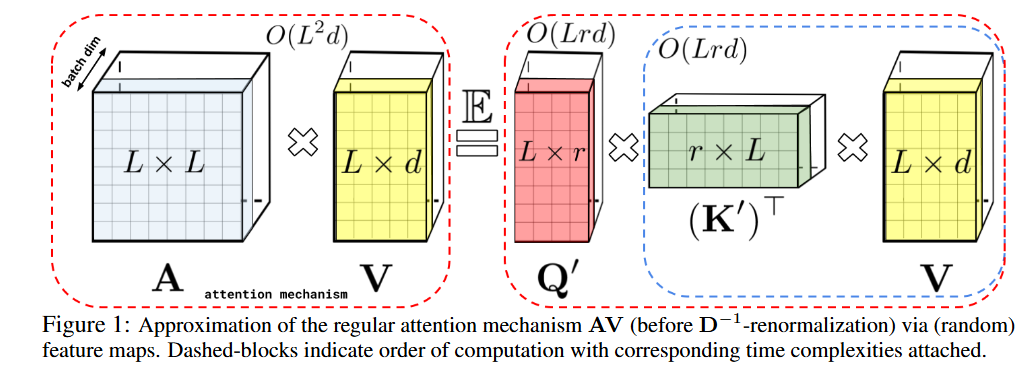

performer

The ultimate choice

The ultimate $\phi(x)$ used for softmax approximation in the Performer is the Positive Random Feature (PRF) map. It combines the $h(x)$ and $f(u)$ functions we discussed into a single, concrete feature mapping.

The paper actually presents two slightly different but related versions of this $\phi(x)$, both derived from Lemma 1 in the paper.

Variant 1: The Standard Positive Feature Map (`SM⁺ₘ`)

This is the most straightforward version, directly implementing the core idea of using exponential functions to ensure positivity.

The ultimate mapping $\phi(x)$ for a single input vector $x$ (which could be a query $q_i$ or a key $k_j$) is:

\[\phi(x) = \exp\left(-\frac{\|x\|^2}{2}\right) \begin{bmatrix} \exp(\omega_1^T x) \\ \exp(\omega_2^T x) \\ \vdots \\ \exp(\omega_r^T x) \end{bmatrix}\]

Let’s break this down:

$\exp(-|x|^2/2)$ : This is the $h(x)$ scaling factor.
$\omega_1, \omega_2, …, \omega_r$ : These are $r$ random vectors drawn from a Gaussian distribution $N(0, I)$. These are the “random features.” For the full FAVOR+ mechanism, these vectors are made orthogonal to each other.
$\exp(\omega_i^T x)$: This is the $f(u)$ function, where $u = \omega_i^Tx$.
The result: The final $\phi(x)$ is a new vector of dimension $r$.

The magic is that the dot product of two such mapped vectors, $\phi(q)^T\phi(k)$, gives an unbiased estimate of the original softmax kernel $\exp(q^Tk)$.

Variant 2: The Variance-Reduced Feature Map (`SM⁺⁺ₘ`)

The paper mentions this second version as a way to “further reduce variance,” meaning it gives a more accurate approximation. It’s based on the hyperbolic cosine (cosh) identity from the derivation in Lemma 1.

The ultimate mapping $\phi(x)$ in this case is:

\[\phi(x) = \frac{1}{\sqrt{2}} \exp\left(-\frac{\|x\|^2}{2}\right) \begin{bmatrix} \exp(\omega_1^T x) \\ \vdots \\ \exp(\omega_r^T x) \\ \exp(-\omega_1^T x) \\ \vdots \\ \exp(-\omega_r^T x) \end{bmatrix}\]

The key differences are:

Two Feature Functions: It uses both $\exp(u)$ and $\exp(-u)$ as feature functions.
Double the Dimension: The resulting feature vector $\phi(x)$ is now in a higher-dimensional space ($2r$ instead of $r$), which helps capture more information and reduce error.
Scaling Factor: A $1/\sqrt2$ scaling factor is introduced to keep the approximation unbiased.

The “Ultimate” Choice

While both are valid, the second variant is theoretically superior due to its lower variance. In practice, the Performer’s FAVOR+ mechanism combines one of these $\phi(x)$ mappings with orthogonal random features ($\omega_i$ are orthogonal) to create the final, highly efficient and accurate linear attention mechanism.

So, the ultimate $\phi$ for softmax approximation is the positive random feature map (ideally the variance-reduced version) where the random projection vectors $\omega_i$ are orthogonalized.

That’s an excellent question that gets to the heart of the “Random Features” method. The notation $\omega_i$ represents the i-th random feature vector. These are the crucial random components that allow the Performer to approximate the complex softmax kernel.

The “choice” of $\omega_i$ involves two main aspects: the distribution they are sampled from, and the relationship between them.

1. The Distribution of each $\omega_i$

For the primary goal of approximating the softmax and Gaussian kernels, each individual random vector $\omega_i$ is drawn from a standard multivariate normal (Gaussian) distribution.

This is written as: $\omega_i \sim \mathcal{N}(0, I_d)$

Let’s break this down:

$\omega_i$: This is a vector with d dimensions, the same as the input query and key vectors (Q and K).
$N$: This signifies a Normal (Gaussian) distribution.
$0$ : The mean of the distribution is the zero vector. This means the random vectors are centered around the origin.
$I_d$: The covariance matrix is the $d \times d$ identity matrix. This is a very important property. It means:
1. Each of the $d$ components within a single vector $\omega_i$ is independent of the others.
2. Each component has a variance of 1.
3. The distribution is isotropic, meaning it’s symmetric around the origin and has no preferred direction. This is a necessary condition for the kernel approximation theory to hold.

2. The Relationship Between Different $\omega_i$ Vectors

This is where the key innovation of FAVOR+ comes in. While each $\omega_i$ comes from the same underlying distribution, you can choose how the different vectors in the set ${\omega_1, \omega_2, …, \omega_r}$ relate to each other.

There are two choices presented in the paper:

Choice A: Independent and Identically Distributed (IID) Sampling This is the standard, baseline approach. You simply draw each of the $r$ vectors from the $N(0, I)$ distribution independently.

Pro: Simple to implement.
Con: The approximation has higher variance, meaning you need a larger $r$ to get a good result, which makes it less efficient.

Choice B: Orthogonal Random Features (ORFs) This is the superior method and the “O” in FAVOR+. The set of $r$ random vectors ${\omega_1, \omega_2, …, \omega_r}$ is constructed to be mutually orthogonal. This means that for any two different vectors $\omega_i$ and $\omega_j$ in the set, their dot product is zero: $\omega_i^T \omega_j = 0 \quad \text{for all } i \neq j$ This is typically achieved by first sampling $r$ vectors independently (like in Choice A) and then applying a procedure like the Gram-Schmidt process to make them orthogonal while preserving the properties of their marginal distribution.

Pro: As proven in Theorem 2, this method provably reduces the variance of the kernel approximation. This means you can achieve the same accuracy with a smaller $r$, making the attention mechanism faster and more memory-efficient.
Con: Slightly more complex to implement due to the extra orthogonalization step.

Summary

The “ultimate” choice of $\omega_i$ for the Performer’s FAVOR+ mechanism is Choice B: Orthogonal Random Features.

So, in summary:

What they are: Each $\omega_i$ is a d-dimensional random vector.
How they are chosen: They are sampled from a standard Gaussian distribution $N(0, I)$ and then are made mutually orthogonal to each other.

Code Snippet

import torch
import torch.nn as nn
import torch.nn.functional as F

class PerformerAttention(nn.Module):
    def __init__(self, d_model: int, num_heads: int, num_random_features: int = 256):
        super().__init__()
        self.num_heads = num_heads
        self.head_dim = d_model // num_heads
        if d_model % num_heads != 0:
            raise ValueError(f"d_model ({d_model}) must be divisible by num_heads ({num_heads})")

        self.query_proj = nn.Linear(d_model, d_model)
        self.key_proj = nn.Linear(d_model, d_model)
        self.value_proj = nn.Linear(d_model, d_model)
        self.out_proj = nn.Linear(d_model, d_model)

        self.num_random_features = num_random_features
        # Random features for queries and keys
        # Omega: (num_heads, head_dim, num_random_features) - fixed during training
        # This is a key difference from standard layers where weights are learnable
        self.register_buffer("omega", torch.randn(num_heads, self.head_dim, num_random_features))

    def _apply_random_features(self, x: torch.Tensor, omega: torch.Tensor):
        # x shape: (batch_size, num_heads, seq_len, head_dim)
        # omega shape: (num_heads, head_dim, num_random_features)
        
        # Project x using random features
        # (batch_size, num_heads, seq_len, head_dim) @ (num_heads, head_dim, num_random_features)
        # -> (batch_size, num_heads, seq_len, num_random_features)
        projection = torch.einsum('bhid,hdo->bhis', x, omega)
        
        # Non-negative feature map (e.g., using exp, or cos/sin pair)
        # A simple non-negative approximation for demonstration:
        # Performer's actual phi is more complex and involves careful normalization.
        phi_x = torch.exp(projection) # or use other forms for robustness
        return phi_x # (batch_size, num_heads, seq_len, num_random_features)

    def forward(self, query: torch.Tensor, key: torch.Tensor, value: torch.Tensor):
        batch_size, q_seq_len, _ = query.size()
        _, kv_seq_len, _ = key.size()

        q = self.query_proj(query)
        k = self.key_proj(key)
        v = self.value_proj(value)

        q = q.view(batch_size, q_seq_len, self.num_heads, self.head_dim).transpose(1, 2)
        k = k.view(batch_size, kv_seq_len, self.num_heads, self.head_dim).transpose(1, 2)
        v = v.view(batch_size, kv_seq_len, self.num_heads, self.head_dim).transpose(1, 2)

        # Apply random feature map to Q and K
        # q_phi, k_phi shapes: (batch_size, num_heads, seq_len, num_random_features)
        q_phi = self._apply_random_features(q, self.omega)
        k_phi = self._apply_random_features(k, self.omega)

        # Compute K_phi^T @ V
        # (batch_size, num_heads, num_random_features, seq_len) @ (batch_size, num_heads, seq_len, head_dim)
        # -> (batch_size, num_heads, num_random_features, head_dim)
        kv_context = torch.matmul(k_phi.transpose(-2, -1), v)

        # Compute unnormalized attention output: Q_phi @ (K_phi^T @ V)
        # (batch_size, num_heads, q_seq_len, num_random_features) @ (batch_size, num_heads, num_random_features, head_dim)
        # -> (batch_size, num_heads, q_seq_len, head_dim)
        unnormalized_attn_output = torch.matmul(q_phi, kv_context)

        # Compute normalization factor: Q_phi @ (K_phi^T @ ones)
        # (batch_size, num_heads, num_random_features, 1) after summing K_phi
        # -> (batch_size, num_heads, q_seq_len, 1)
        k_phi_sum = torch.sum(k_phi, dim=-2, keepdim=True) # sum over sequence length of k_phi
        normalization_factor = torch.matmul(q_phi, k_phi_sum.transpose(-2,-1))
        
        epsilon = 1e-6
        normalized_attn_output = unnormalized_attn_output / (normalization_factor + epsilon)

        # Reshape and final projection
        output = normalized_attn_output.transpose(1, 2).contiguous().view(batch_size, q_seq_len, self.num_heads * self.head_dim)
        output = self.out_proj(output)
        return output

# Example Usage
if __name__ == "__main":
    batch_size = 2
    seq_len = 1024
    d_model = 256
    num_heads = 4
    num_random_features = 256 # This M dimension is crucial for Performer

    query = torch.randn(batch_size, seq_len, d_model)
    key = torch.randn(batch_size, seq_len, d_model)
    value = torch.randn(batch_size, seq_len, d_model)

    performer_attn = PerformerAttention(d_model, num_heads, num_random_features=num_random_features)
    output_performer = performer_attn(query, key, value)
    print(f"Performer Attention output shape: {output_performer.shape}") # (2, 1024, 256)

4. Advantages of Performer

Aspect	Performer (FAVOR+)
Complexity	$O(n d)$ linear w.r.t sequence length
Accuracy	High-fidelity approximation to softmax attention
Memory usage	Constant with respect to sequence length
Theory	Grounded in Bochner’s theorem and RFF
GPU/TPU friendly	Matrix multiplications only, no loops or recursions

5. Summary

Kernels let us measure similarity implicitly in high dimensions.
Bochner’s theorem enables us to write shift-invariant kernels as expectations over Fourier features.
Monte Carlo approximations yield explicit feature maps.
RBF kernel cannot be represented in finite dimensions, so we approximate it using sampled random Fourier bases.
Performer uses this machinery to linearize attention, scaling Transformers to long sequences efficiently.

Kernel-Based Attention and the Performer: Full Tutorial

1. What Is a Kernel?

Examples of Kernels and Their Feature Maps

2. Random Fourier Features (RFF)

Reduce dimensionality using random phase shifts

Monte Carlo Approximation

Why This Works

Note on RBF Kernel and Infinite Dimensions

Unified View: Kernel Approximations via Random Features

3. Softmax Kernel Approximation (via Gaussian MGF Trick)

① Kernel:

Moment-Generating Function (MGF) of Gaussian:

③ Rearranged:

Final Feature Map (Performer-style):

Comparison Table

4. Performer: FAVOR+ Attention

Step-by-Step Performer Attention

Final Output:

The ultimate choice

Variant 1: The Standard Positive Feature Map (SM⁺ₘ)

Variant 2: The Variance-Reduced Feature Map (SM⁺⁺ₘ)

The “Ultimate” Choice

1. The Distribution of each $\omega_i$

2. The Relationship Between Different $\omega_i$ Vectors

Summary

Code Snippet

4. Advantages of Performer

5. Summary

Variant 1: The Standard Positive Feature Map (`SM⁺ₘ`)

Variant 2: The Variance-Reduced Feature Map (`SM⁺⁺ₘ`)