A Deep Dive into Multi-Query and Grouped-Query Attention (MQA & GQA)

The Transformer architecture’s self-attention mechanism is the engine of modern AI. However, as models and their context windows grow, the computational and memory costs of standard Multi-Head Attention (MHA) become a significant bottleneck, especially during inference.

This tutorial provides an in-depth exploration of two powerful solutions: Multi-Query Attention (MQA) and Grouped-Query Attention (GQA). Understanding these architectural details, including their mathematical foundations and impact on memory, is essential for grasping how models like Google’s Gemini, Meta’s Llama 3, and Mistral AI’s models operate so efficiently.

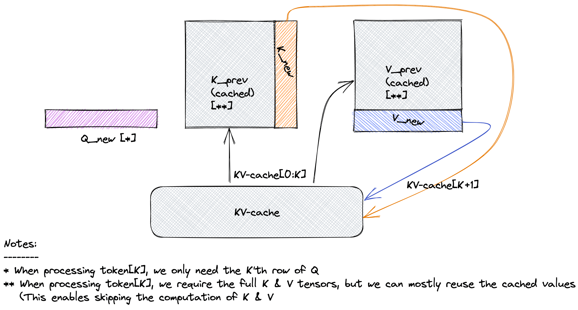
Fig.1: KV caching in the sequence2sequence Transformer architectures

A Deeper Look at the KV Cache

To understand MQA and GQA, one must first understand the KV Cache.

During autoregressive decoding (generating text token by token), the model needs to “look back” at all previously generated tokens to decide the next one. Let’s say we are generating the $t$-th token. Its Query vector, $q_t$, must attend to the Key and Value vectors of all previous tokens, ${k_1, v_1}, {k_2, v_2}, \dots, {k_{t-1}, v_{t-1}}$, as well as its own, ${k_t, v_t}$.

Without a cache, at each step $t$, we would have to re-calculate the K and V vectors for all preceding $t-1$ tokens. This is incredibly redundant and inefficient.

The KV Cache solves this by storing the Key and Value vectors for all tokens in the context window as they are generated. At step $t$, we simply calculate $k_t$ and $v_t$, append them to our cache, and perform the attention calculation using the full cache.

The bottleneck then shifts from computation to memory bandwidth. At every single generation step, the entire KV cache must be loaded from slow High-Bandwidth Memory (HBM) into the fast on-chip SRAM of the processor. This memory transfer is the primary factor limiting inference speed. The goal of MQA and GQA is to shrink this cache.

---

Part 1: Revisiting Multi-Head Attention (MHA)

MHA is the foundational attention mechanism.

• Mathematical Formulation: Given an input sequence representation $X \in \mathbb{R}^{n \times d_{model}}$, MHA first projects it into $H$ sets of queries, keys, and values using distinct weight matrices for each head $i \in {1, \dots, H}$:
  • Query: $Q_i = X W_i^Q$, where $W_i^Q \in \mathbb{R}^{d_{model} \times d_k}$
  • Key: $K_i = X W_i^K$, where $W_i^K \in \mathbb{R}^{d_{model} \times d_k}$
  • Value: $V_i = X W_i^V$, where $W_i^V \in \mathbb{R}^{d_{model} \times d_v}$

  The output of each head is then calculated, concatenated, and projected back: \(\text{head}_i = \text{Attention}(Q_i, K_i, V_i) = \text{softmax}\left(\frac{Q_i K_i^T}{\sqrt{d_k}}\right)V_i\) \(\text{MHA}(X) = \text{Concat}(\text{head}_1, \dots, \text{head}_H)W^O\)

• KV Cache Size: The total size is determined by the Key and Value tensors across all heads and layers. \(C_{MHA} = 2 \times B \times L \times N_{layers} \times H \times d_k\) Where:
  • 2: For storing both K and V tensors.
  • B: Batch size.
  • L: Sequence length.
  • N_layers: Number of transformer layers.
  • H: Number of attention heads.
  • d_k: Dimension of each head.

---

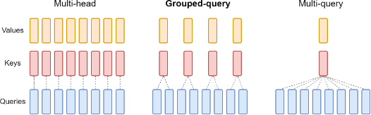
Fig. 2 Overview of grouped-query method. Multi-head attention has H query, key, and value heads. Multi-query attention shares single key and value heads across all query heads. Grouped-query attention instead shares single key and value heads for each group of query heads, interpolating between multi-head and multi-query attention.

Part 2: Multi-Query Attention (MQA)

MQA aggressively shrinks the KV cache by sharing one K/V head across all query heads.

• Mathematical Formulation: MQA retains $H$ distinct Query heads but uses only a single Key and Value projection matrix. Given input $X \in \mathbb{R}^{L \times d_{model}}$:
  • Query: $Q_i = X W_i^Q$ (for $i=1, \dots, H$), where $W_i^Q \in \mathbb{R}^{d_{model} \times d_k}$. This results in $H$ distinct query tensors, each $Q_i \in \mathbb{R}^{L \times d_k}$.
  • Key: $K = X W^K$, where $W^K \in \mathbb{R}^{d_{model} \times d_k}$. This results in a single key tensor $K \in \mathbb{R}^{L \times d_k}$.
  • Value: $V = X W^V$, where $W^V \in \mathbb{R}^{d_{model} \times d_v}$. This results in a single value tensor $V \in \mathbb{R}^{L \times d_v}$.

  The attention calculation for each head then uses the same K and V: \(\text{head}_i = \text{Attention}(Q_i, K, V) = \text{softmax}\left(\frac{Q_i K^T}{\sqrt{d_k}}\right)V\)

• KV Cache Reduction: When calculating the total memory, we include the batch size B. Since there is only one K/V head, the cache size formula becomes: \(C_{MQA} = 2 \times B \times L \times N_{layers} \times \mathbf{1} \times d_k\) The reduction factor compared to MHA is simply the number of heads, $H$. \(\frac{C_{MHA}}{C_{MQA}} = H\) For a model with 32 attention heads, MQA reduces the KV cache size by a factor of 32, leading to a massive speedup in inference.

• Code Snippet (PyTorch): This code correctly handles a batch of sequences.

    import torch
    import torch.nn as nn
  
    class MultiQueryAttention(nn.Module):
        def __init__(self, d_model, num_heads):
            super().__init__()
            assert d_model % num_heads == 0
            self.d_model = d_model
            self.num_heads = num_heads
            self.d_head = d_model // num_heads
  
            self.q_proj = nn.Linear(d_model, d_model) # Projects all Q heads at once
            # Only one projection for K and one for V
            self.k_proj = nn.Linear(d_model, self.d_head)
            self.v_proj = nn.Linear(d_model, self.d_head)
            self.out_proj = nn.Linear(d_model, d_model)
  
        def forward(self, x):
            batch_size, seq_len, _ = x.shape
  
            # Project and reshape Q into H heads
            q = self.q_proj(x).view(batch_size, seq_len, self.num_heads, self.d_head).transpose(1, 2)
            # Project K and V (result has no head dimension yet)
            k = self.k_proj(x).view(batch_size, seq_len, 1, self.d_head).transpose(1, 2)
            v = self.v_proj(x).view(batch_size, seq_len, 1, self.d_head).transpose(1, 2)
  
            # Attention calculation is now broadcast-compatible
            # Q: (B, H, L, d_k), K.T: (B, 1, d_k, L) -> Scores: (B, H, L, L)
            scores = torch.matmul(q, k.transpose(-2, -1)) / (self.d_head ** 0.5)
            attn = torch.softmax(scores, dim=-1)
  
            # V: (B, 1, L, d_k)
            output = torch.matmul(attn, v) # Output: (B, H, L, d_k)
              
            # Concatenate heads and project out
            output = output.transpose(1, 2).contiguous().view(batch_size, seq_len, self.d_model)
            return self.out_proj(output)
  

  ---

Part 3: Grouped-Query Attention (GQA)

GQA provides a balance, grouping Query heads and assigning a single K/V head to each group.

Detailed Mechanics of GQA

Let’s break down exactly how the query grouping, attention, and concatenation works using a concrete example. Imagine a model with:

• H = 8 total Query heads.
• G = 2 Key/Value heads (i.e., 2 KV groups).

This means there are H / G = 4 Query heads per group.

1. Grouping Queries and Assigning KV Heads (The “Many-to-One” Mapping)

First, the H Query heads are conceptually partitioned into G groups.

• Group 1: Consists of Query_1, Query_2, Query_3, Query_4.
• Group 2: Consists of Query_5, Query_6, Query_7, Query_8.

Simultaneously, we have our G=2 Key and Value heads, KV_1 and KV_2. The core idea of GQA is that every query in a group attends to the same KV head assigned to that group.

• All queries in Group 1 (Q1 to Q4) will perform attention using K1 and V1.
• All queries in Group 2 (Q5 to Q8) will perform attention using K2 and V2.

Implementation Trick: Instead of running four separate attention calculations for Group 1, this is done in a single, efficient operation. The K1 and V1 tensors are “repeated” or “broadcast” four times to match the shape of the four Q-heads. This is what the repeat_interleave function in the code snippet does. It’s a highly optimized way to perform this sharing without inefficient loops or memory copies.

2. Concatenation and Final Output (The “Reunification”)

This step is identical to standard Multi-Head Attention. This is a critical point: GQA’s innovation is entirely on the Key/Value side before the main attention calculation. The processing after attention is unchanged.

1. Get Head Outputs: After the attention step, we have H=8 distinct output vectors (head_1 through head_8), each representing what its corresponding Query “learned” from its assigned KV group. Each head_i has a dimension of d_v.
2. Concatenate: All H of these output vectors are concatenated together along their feature dimension. So, if each head output is a tensor of shape (L, d_v), concatenating all 8 results in a single, wide tensor of shape (L, H * d_v).
3. Final Projection: This wide tensor, containing the mixed knowledge from all heads, is passed through a final linear projection layer (W^O). This layer mixes the information from all heads and maps the dimension back to the model’s expected dimension, d_model (since H * d_v = d_model).

So, despite the complex sharing mechanism on the input side, the output side reunifies all H query pathways in the exact same way as MHA.

Mathematical Formulation

Given input $X \in \mathbb{R}^{L \times d_{model}}$:

• Query: $Q_i = X W_i^Q$ (for $i=1, \dots, H$), resulting in $H$ tensors $Q_i \in \mathbb{R}^{L \times d_k}$.
• Key: $K_g = X W_g^K$ (for $g=1, \dots, G$), resulting in $G$ tensors $K_g \in \mathbb{R}^{L \times d_k}$.
• Value: $V_g = X W_g^V$ (for $g=1, \dots, G$), resulting in $G$ tensors $V_g \in \mathbb{R}^{L \times d_v}$.

The attention for head $i$ uses the K and V from its assigned group $g(i)$: \(\text{head}_i = \text{Attention}(Q_i, K_{g(i)}, V_{g(i)})\)

KV Cache Reduction

With $G$ Key/Value heads, the total cache size is: \(C_{GQA} = 2 \times B \times L \times N_{layers} \times \mathbf{G} \times d_k\) The reduction factor compared to MHA is the number of heads per group. \(\frac{C_{MHA}}{C_{GQA}} = \frac{H}{G}\) For example, a model like Llama 2 7B uses $H=32$ Query heads and $G=4$ KV heads. The KV cache is reduced by a factor of $32/4 = 8$.

Code Snippet (PyTorch)

import torch
import torch.nn as nn

class GroupedQueryAttention(nn.Module):
    def __init__(self, d_model, num_heads, num_kv_heads):
        super().__init__()
        assert d_model % num_heads == 0
        assert num_heads % num_kv_heads == 0
        self.d_model = d_model
        self.num_heads = num_heads
        self.num_kv_heads = num_kv_heads
        self.num_queries_per_kv = num_heads // num_kv_heads
        self.d_head = d_model // num_heads

        self.q_proj = nn.Linear(d_model, d_model)
        # K and V projections are smaller now
        self.k_proj = nn.Linear(d_model, self.num_kv_heads * self.d_head)
        self.v_proj = nn.Linear(d_model, self.num_kv_heads * self.d_head)
        self.out_proj = nn.Linear(d_model, d_model)

    def forward(self, x):
        batch_size, seq_len, _ = x.shape

        # Project Q, K, V
        q = self.q_proj(x).view(batch_size, seq_len, self.num_heads, self.d_head).transpose(1, 2)
        k = self.k_proj(x).view(batch_size, seq_len, self.num_kv_heads, self.d_head).transpose(1, 2)
        v = self.v_proj(x).view(batch_size, seq_len, self.num_kv_heads, self.d_head).transpose(1, 2)
        
        # Repeat K and V heads to match the number of Q heads in each group
        # From (B, G, L, d_k) to (B, H, L, d_k)
        k = k.repeat_interleave(self.num_queries_per_kv, dim=1)
        v = v.repeat_interleave(self.num_queries_per_kv, dim=1)

        # Attention calculation
        scores = torch.matmul(q, k.transpose(-2, -1)) / (self.d_head ** 0.5)
        attn = torch.softmax(scores, dim=-1)
        output = torch.matmul(attn, v)
        
        output = output.transpose(1, 2).contiguous().view(batch_size, seq_len, self.d_model)
        return self.out_proj(output)

---

Comparison Summary

Feature	Multi-Head (MHA)	Grouped-Query (GQA)	Multi-Query (MQA)
# Q Heads	H	H	H
# K/V Heads	H	G (where 1 < G < H)	1
KV Cache Reduction Factor	1x (Baseline)	H / G	H
Inference Speed	Slowest	Fast	Fastest
Model Quality	Highest (Baseline)	Nearly as high as MHA	Can be slightly lower
Best For	Max performance (if memory allows)	The modern standard for LLMs	Extreme memory constraints

Conclusion

The evolution from MHA to GQA is a story of pragmatic engineering. GQA masterfully balances the expressive power of having many attention heads with the practical necessity of a small memory footprint for fast inference. By grouping query heads, it achieves most of the speed benefits of MQA while retaining nearly all the model quality of MHA, solidifying its place as a cornerstone of today’s state-of-the-art language models.

---

References

1. GQA (Canonical Paper): Ainslie, J., Lee-Thorp, J., de Jong, M., Zemlyanskiy, Y., Le, Q., & Sanghai, S. (2023). GQA: Training Generalized Multi-Query Transformer Models from Multi-Head Checkpoints. arXiv preprint arXiv:2305.13245.
2. MQA (Conceptual Origin): Shazeer, N. (2019). Fast Transformer Decoding: One Write-Head is All You Need. arXiv preprint arXiv:1911.02150.
3. Original Transformer (Foundation): Vaswani, A., Shazeer, N., Parmar, N., Uszkoreit, J., Jones, L., Gomez, A. N., Kaiser, Ł., & Polosukhin, I. (2017). Attention Is All You Need. Advances in Neural Information Processing Systems 30 (NIPS 2017).