Linformer

What is Low-Rank Attention?

In standard self-attention, the core operation involves computing the attention matrix $A = QK^T$, where $Q, K \in \mathbb{R}^{L \times d_k}$. This matrix $A$ has dimensions $L \times L$. The rank of this matrix can be at most $\min(L, d_k)$. If $d_k < L$ (which is very common, as $d_k = d_{model}/h$ and $d_{model}$ is usually much smaller than $L$ for long sequences), then the attention matrix $A$ is inherently low-rank (its rank is at most $d_k$).

Low-rank attention methods explicitly leverage or enforce this property to reduce computational and memory costs. They aim to approximate the full $L \times L$ attention matrix with a matrix that can be represented and computed more efficiently due to its lower rank.

Why Low-Rank? Motivation

The primary motivations for using low-rank attention are:

Computational Efficiency:
- Calculating $QK^T$ takes $O(L^2 d_k)$ operations.
- Multiplying this $L \times L$ attention matrix by $V \in \mathbb{R}^{L \times d_v}$ takes $O(L^2 d_v)$ operations.
- By forcing or exploiting a lower rank, we can bypass the direct computation of the full $L \times L$ matrix, leading to reduced complexity.
Memory Efficiency:
- Storing the attention matrix $QK^T$ requires $O(L^2)$ memory. For very long sequences, this quickly becomes prohibitive.
- Low-rank approximations can drastically reduce memory usage by storing only the factors of the low-rank decomposition.
Regularization (Implicit):
- Restricting the expressiveness of the attention matrix to a lower rank can sometimes act as a form of regularization, potentially preventing overfitting on smaller datasets or encouraging learning more general patterns.

Mathematical Foundation: Low-Rank Matrix Approximation

A fundamental concept in linear algebra is that any matrix $M \in \mathbb{R}^{N \times M}$ can be approximated by a lower-rank matrix $M’ \in \mathbb{R}^{N \times M}$ if $M’$ can be written as the product of two thinner matrices: $M' = UV^T$ where $U \in \mathbb{R}^{N \times r}$ and $V \in \mathbb{R}^{M \times r}$ (or $V^T \in \mathbb{R}^{r \times M}$), and $r < \min(N, M)$. The rank of $M’$ is at most $r$.

The key idea for low-rank attention is to either: a. Implicitly exploit the fact that $QK^T$ already has a low rank (at most $d_k$) if $d_k < L$. b. Explicitly construct $Q, K, V$ or intermediate matrices such that the effective attention matrix is low-rank, often by projecting the sequence length $L$ down to a smaller dimension $k$ before the main attention calculation.

How is it Achieved in Attention?

a) Implicit Low-Rank via $d_k$

As mentioned, the matrix $QK^T \in \mathbb{R}^{L \times L}$ has a maximum rank of $d_k$ (the dimension of keys/queries). If $d_k \ll L$, then the attention matrix is already inherently low-rank.

In this case, the efficiency gain primarily comes from reordering the operations in the attention calculation, as seen in some “linear attention” methods (which also happen to be kernel-based). For example, in the $O(L \cdot d^2)$ formulations (like Linear Attention or Performer): $\text{Attention}(Q, K, V) = \text{Norm}(\phi(Q) (\phi(K)^T V))$ Here, $(\phi(K)^T V)$ is a $d_k \times d_v$ matrix. Its computation takes $O(L d_k d_v)$. The subsequent multiplication $\phi(Q) (\phi(K)^T V)$ takes $O(L d_k d_v)$. The $L^2$ term is avoided because we never explicitly form the $L \times L$ matrix. The rank of the implicit attention matrix might still be $d_k$, but the computation avoids the $L^2$ part.

b) Explicit Low-Rank Decomposition (e.g., Linformer)

Some methods directly aim to reduce the effective sequence length (or rank) before computing the attention. The most prominent example here is Linformer.

Linformer: A Primary Example of Explicit Low-Rank Attention

Linformer (Wang et al., 2020) explicitly projects the input sequence length $L$ down to a much smaller constant $k$ (where $k \ll L$) before computing the dot-product attention. This effectively forces the attention matrix to be of rank at most $k$.

Intuition:

Instead of asking each token to compute attention with every other token, Linformer suggests that perhaps each token only needs to attend to a small, compressed representation of the entire sequence. This “compressed representation” is created by linearly projecting the keys and values from $L$ length down to $k$ length.

Imagine taking a very long document and summarizing it into $k$ key sentences. Then, when a word in the original document needs context, it attends to these $k$ summarized sentences, rather than the entire original document.

Linformer

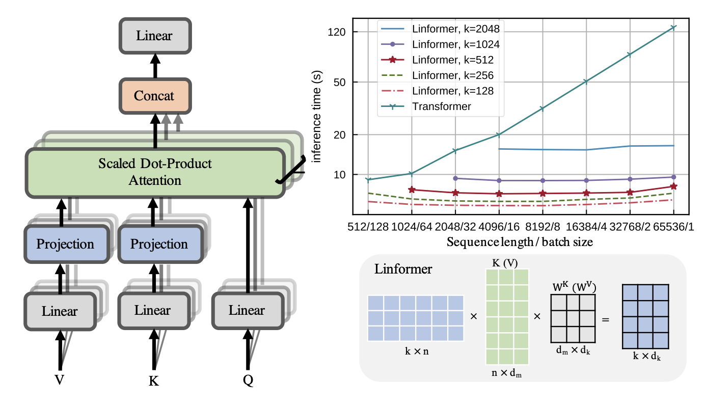
Fig. 1: Linformer architecture along with its performance for different values of $K$

Mathematical Description:

For each attention head, given input $X \in \mathbb{R}^{L \times d_{model}}$, the standard Transformer first projects it to $Q, K, V \in \mathbb{R}^{L \times d_k}$ (or $d_v$).

Linformer introduces two additional learnable projection matrices, $E \in \mathbb{R}^{L \times k}$ and $F \in \mathbb{R}^{L \times k}$, which act on the sequence length dimension:

Project Keys: The original keys $K \in \mathbb{R}^{L \times d_k}$ are projected using $E$: $K’ = E^T K$ Where $E^T \in \mathbb{R}^{k \times L}$ and $K \in \mathbb{R}^{L \times d_k}$. So, $K’ \in \mathbb{R}^{k \times d_k}$. This means the effective sequence length for keys becomes $k$.
Project Values: Similarly, the original values $V \in \mathbb{R}^{L \times d_v}$ are projected using $F$: $V’ = F^T V$ Where $F^T \in \mathbb{R}^{k \times L}$ and $V \in \mathbb{R}^{L \times d_v}$. So, $V’ \in \mathbb{R}^{k \times d_v}$. The effective sequence length for values also becomes $k$.
Attention Calculation: Now, the attention is computed with the original Queries $Q \in \mathbb{R}^{L \times d_k}$ and the projected Keys $K’ \in \mathbb{R}^{k \times d_k}$ and Values $V’ \in \mathbb{R}^{k \times d_v}$: $\text{Attention}(Q, K', V') = \text{softmax}\left(\frac{Q (K')^T}{\sqrt{d_k}}\right) V'$
- $Q \in \mathbb{R}^{L \times d_k}$ and $(K’)^T \in \mathbb{R}^{d_k \times k}$. Their product $Q(K’)^T$ is $\mathbb{R}^{L \times k}$.
- This $L \times k$ matrix is then passed through softmax (row-wise).
- The result is multiplied by $V’ \in \mathbb{R}^{k \times d_v}$. The final output is $\mathbb{R}^{L \times d_v}$.

Complexity Analysis:

Let’s break down the computational steps and their complexities for Linformer:

Key Projection ($K’$): $E^T K$. $E^T \in \mathbb{R}^{k \times L}$, $K \in \mathbb{R}^{L \times d_k}$.
- Complexity: $O(k \cdot L \cdot d_k)$.
Value Projection ($V’$): $F^T V$. $F^T \in \mathbb{R}^{k \times L}$, $V \in \mathbb{R}^{L \times d_v}$.
- Complexity: $O(k \cdot L \cdot d_v)$.
Dot Product ($Q(K’)^T$): $Q \in \mathbb{R}^{L \times d_k}$, $(K’)^T \in \mathbb{R}^{d_k \times k}$.
- Complexity: $O(L \cdot d_k \cdot k)$.
Softmax: Applied to an $L \times k$ matrix.
- Complexity: $O(L \cdot k)$.
Weighted Sum ($(L \times k) \cdot (k \times d_v)$):
- Complexity: $O(L \cdot k \cdot d_v)$.

Total Complexity for one head: $O(k \cdot L \cdot d_k + k \cdot L \cdot d_v + L \cdot d_k \cdot k + L \cdot k \cdot d_v)$. Assuming $d_k \approx d_v \approx d_{model}/h = d’$, this simplifies to $O(L \cdot k \cdot d’)$.

Since $k$ is a small constant (e.g., $k=256$ even for $L=32768$), the complexity becomes $O(L \cdot d’ \cdot \text{const})$ or simply $O(L \cdot d’)$. This is linear with respect to sequence length $L$.

Memory Complexity:

Storing $Q, K, V$: $O(L \cdot d)$
Storing $K’, V’$: $O(k \cdot d)$
Storing the attention matrix $Q(K’)^T$: $O(L \cdot k)$
Overall memory complexity: $O(L \cdot d + L \cdot k)$, which is dominated by $O(L \cdot d)$ for long sequences.

Key Advantages of Linformer:

True Linear Complexity: Achieves strict linear complexity $O(L)$ for large $L$ by making $k$ a fixed constant.
Simplicity: The change is relatively straightforward: add two linear projection layers.
Performance: Demonstrates competitive performance against standard Transformers on various tasks while being much faster for long sequences.

Limitations:

The fixed size $k$ might act as a bottleneck for extremely complex long-range dependencies where a truly high-rank attention might be beneficial.
The projection matrices $E$ and $F$ need to be learned effectively.

Why only project K and V and not Q?

The fundamental reason is both mathematical and conceptual: you need to generate an output for every token in the sequence, and the Query (Q) is what drives this process for each individual token.

Let’s break this down into a conceptual reason and a mathematical one.

1. The Conceptual Reason: The Role of Q, K, and V

Think of the attention mechanism as a search in a library for each word in your sentence.

Query (Q): This is your search query. For every single token in the input sequence, you generate a unique Query. It’s the token that is actively “looking for” context from the rest of the sequence. If you have a sequence of n tokens, you must have n queries to produce n updated tokens.
Key (K): This is like the card catalog or index of the library. Each token in the sequence has a Key that says, “this is the kind of information I represent.”
Value (V): This is the actual content of the books on the shelves. Each token has a Value that contains its informational content.

The core hypothesis of Linformer is that you don’t need to check the entire, highly-detailed card catalog (K) and read every single book (V) to get the necessary context. You can create a compressed summary of the library’s contents.

Projecting K and V: This is like creating a “CliffsNotes” or a summarized index of the library. You are reducing the n key-value pairs to a smaller, representative set of k key-value pairs. This summary still captures the most important information from the full sequence.
Why NOT Project Q: You still need to perform the search for every single one of your original n tokens. Each token needs to take its unique query, compare it against the summarized library (the projected K), and then retrieve information from the summarized content (the projected V). If you were to project the Queries down to k queries, you would only be asking k questions and would therefore only get k outputs. The goal of a self-attention layer is to update all n tokens, not just a small subset.

Projecting Q would mean losing the one-to-one mapping between input tokens and output tokens, which would fundamentally break the structure of the Transformer.

2. We Still Need an Output Token for Each Position ($L$)

The output of the attention mechanism is still $(B, L, d)$, meaning we produce a new embedding for each of the $L$ tokens.
The Query dimension (the “rows” of the attention matrix) corresponds directly to the number of tokens ($L$) for which we want to compute an updated representation.
If we also projected $Q$ down to size $k$, we would effectively reduce the number of output tokens from $L$ to $k$, which is not what we want—each position in the input still needs its own separate query and

3. The Mathematical Reason: Breaking the Bottleneck

The computational bottleneck in standard self-attention is the matrix multiplication of Q and K^T.

Let’s look at the matrix dimensions:

Q has shape (n, d_k) (sequence length x dimension of key)
K has shape (n, d_k)
V has shape (n, d_v) (sequence length x dimension of value)

The bottleneck operation is Q @ K.transpose(-1, -2), which results in an (n, n) attention matrix. The complexity is $O(n^2)$, which is very expensive for long sequences.

Linformer’s Approach:

Linformer introduces a projection matrix E of shape (k, n) that projects the sequence dimension n down to a smaller, fixed dimension k.

Project K and V:
- K_proj = E @ K –> resulting effective shape is (k, d_k)
- V_proj = E @ V –> resulting effective shape is (k, d_v)
Perform Attention:
- First multiplication: Q @ K_proj.transpose(-1, -2)
  - Dimensions: (n, d_k) @ (d_k, k) -> (n, k)
  - This creates a much smaller attention-like score matrix. The complexity is now $O(n \cdot k \cdot d_k)$, which is linear with respect to n.
- Second multiplication: (n, k) @ V_proj
  - Dimensions: (n, k) @ (k, d_v) -> (n, d_v)
  - This produces the final output with the correct shape, where each of the n tokens has an updated representation.

What if we projected Q instead?

If you projected Q to Q_proj (shape k, d_k) and used the full K, your first multiplication would be Q_proj @ K.transpose, resulting in a (k, n) matrix. The final output after multiplying with V would have a sequence length of k, not n. You would have failed to compute an output for every input token.

In summary: The low-rank approximation is applied to the Key and Value matrices because they represent the global “context” or “information source” of the entire sequence, which can be effectively summarized. The Query matrix is left untouched because it represents the specific, individual need of each token in the sequence to gather that context, and you must preserve one query per token to get one output per token.

Code Snippet (Conceptual Linformer Attention Module)

import torch
import torch.nn as nn
import math

class LinformerAttention(nn.Module):
    """
    Implements Linformer attention, which reduces the complexity of the attention
    mechanism from O(n^2) to O(n*k) by projecting the Key (K) and Value (V)
    matrices to a lower-dimensional space.
    """
    def __init__(self, dim, heads, k, dropout=0.1):
        """
        Args:
            dim (int): The input dimension of the model.
            heads (int): The number of attention heads.
            k (int): The projected dimension for keys and values. This is the
                     bottleneck dimension and the key to Linformer's efficiency.
            dropout (float): The dropout rate.
        """
        super().__init__()
        assert dim % heads == 0, 'dimension must be divisible by heads'

        self.heads = heads
        self.k = k
        self.dim_head = dim // heads
        self.scale = self.dim_head ** -0.5 # For scaled dot-product attention

        # Linear layers for Q, K, V
        self.to_q = nn.Linear(dim, dim, bias=False)
        self.to_k = nn.Linear(dim, dim, bias=False)
        self.to_v = nn.Linear(dim, dim, bias=False)

        # Projection matrices for K and V
        # These project the sequence length 'n' down to 'k'
        self.proj_k = nn.Linear(self.dim_head, self.k)
        self.proj_v = nn.Linear(self.dim_head, self.k)

        self.dropout = nn.Dropout(dropout)
        self.to_out = nn.Linear(dim, dim)

    def forward(self, x, mask=None):
        """
        Forward pass for Linformer attention.

        Args:
            x (torch.Tensor): Input tensor of shape (batch_size, seq_len, dim).
            mask (torch.Tensor, optional): Attention mask. Not typically used
                                           in Linformer's original formulation but
                                           included for completeness.
        
        Returns:
            torch.Tensor: Output tensor of shape (batch_size, seq_len, dim).
        """
        batch_size, seq_len, _ = x.shape

        # 1. Project to Q, K, V and split into heads
        # (batch_size, seq_len, heads, dim_head) -> (batch_size, heads, seq_len, dim_head)
        q = self.to_q(x).view(batch_size, seq_len, self.heads, self.dim_head).transpose(1, 2)
        k = self.to_k(x).view(batch_size, seq_len, self.heads, self.dim_head).transpose(1, 2)
        v = self.to_v(x).view(batch_size, seq_len, self.heads, self.dim_head).transpose(1, 2)

        # 2. Project K and V to lower dimension 'k'
        # Transpose to (batch_size, heads, dim_head, seq_len) for linear projection
        k = k.transpose(-1, -2) # Becomes (batch_size, heads, dim_head, seq_len)
        v = v.transpose(-1, -2) # Becomes (batch_size, heads, dim_head, seq_len)
        
        # Apply the projection E
        k_proj = self.proj_k(k) # (batch_size, heads, dim_head, k)
        v_proj = self.proj_v(v) # (batch_size, heads, dim_head, k)

        # Transpose back to be compatible with Q
        k_proj = k_proj.transpose(-1, -2) # (batch_size, heads, k, dim_head)
        v_proj = v_proj.transpose(-1, -2) # (batch_size, heads, k, dim_head)

        # 3. Calculate attention with projected K
        # (batch, heads, seq_len, dim_head) @ (batch, heads, dim_head, k) -> (batch, heads, seq_len, k)
        attn_scores = torch.matmul(q, k_proj.transpose(-1, -2)) * self.scale
        attn_probs = attn_scores.softmax(dim=-1)
        attn_probs = self.dropout(attn_probs)

        # 4. Apply attention to projected V
        # (batch, heads, seq_len, k) @ (batch, heads, k, dim_head) -> (batch, heads, seq_len, dim_head)
        context = torch.matmul(attn_probs, v_proj)

        # 5. Concatenate heads and project out
        # (batch, heads, seq_len, dim_head) -> (batch, seq_len, heads * dim_head)
        context = context.transpose(1, 2).contiguous().view(batch_size, seq_len, -1)
        
        return self.to_out(context)

# --- Usage Example ---
if __name__ == '__main__':
    # Model parameters
    input_dim = 512    # Dimension of the model (e.g., word embedding size)
    num_heads = 8      # Number of attention heads
    seq_length = 4096  # Original sequence length (long)
    projected_k = 256  # Projected sequence length (much shorter)
    batch_size = 4

    # Create a random input tensor
    input_tensor = torch.randn(batch_size, seq_length, input_dim)

    # Instantiate the Linformer attention module
    linformer_attn = LinformerAttention(
        dim=input_dim,
        heads=num_heads,
        k=projected_k
    )

    # Get the output
    output = linformer_attn(input_tensor)

    print(f"Input Shape:  {input_tensor.shape}")
    print(f"Output Shape: {output.shape}")
    
    # Verify that the output shape is the same as the input shape
    assert input_tensor.shape == output.shape
    print("\n✅ The output shape is correct.")