# K-Means Clustering and k-means++ Initialization: A Practical Tutorial

🔍 Overview

K-Means is a popular clustering algorithm used to partition a dataset into K clusters by minimizing intra-cluster variance. A crucial factor in its performance is how you initialize the cluster centroids. This tutorial covers:

• The mechanics of K-Means and k-means++ initialization
• How to choose the right number of clusters

• Best practices to avoid centroid collapse

🔧 K-Means Algorithm

Given a dataset $X = {x_1, x_2, \ldots, x_n} \subset \mathbb{R}^d$, K-Means partitions the data into $K$ clusters ${C_1, \ldots, C_K}$ by minimizing the total within-cluster sum of squares:

📌 Inertia (Objective Function)

The quantity minimized in k-means is called inertia:

\[\text{Inertia} = \sum_{i=1}^{K} \sum_{x_j \in C_i} \|x_j - c_i\|^2\]

Where $c_i$ is the centroid of cluster $C_i$.

---

✅ k-means++ Initialization

📁 Problem with Random Initialization

Randomly selecting $K$ centroids can cause poor convergence, centroid collapse, or suboptimal clustering.

🔎 k-means++ Algorithm

A better strategy is k-means++, which chooses centroids to be diverse and far apart. Here’s the step-by-step:

1. Choose the first centroid $c_1 \in X$ randomly.

2. For each remaining centroid $c_k$:

   • For every $x \in X$, compute: $D(x)^2 = \min_{1 \leq j < k} |x - c_j|^2$
   • Sample next centroid with probability: $P(x) = \frac{D(x)^2}{\sum_{x’ \in X} D(x’)^2}$
3. Repeat until $K$ centroids are selected.
4. Proceed with regular Lloyd’s algorithm.

⚡ Benefits

• Strong theoretical guarantees: expected cost $\leq 8(\log K + 2) \cdot \text{OPT}$
• Prevents collapse and encourages diverse cluster initialization

---

🧪 Python Code Example

Here’s a simple k-means implementation using NumPy with inline shape comments:

import numpy as np

def initialize_kmeans_plusplus(X, K):
    # X: (n_samples, n_features)
    n_samples = X.shape[0]
    centroids = [X[np.random.randint(n_samples)]]  # first centroid: (n_features,)

    for _ in range(1, K):
        # dists: (n_samples,), each element is D(x)^2
        dists = np.array([min(np.linalg.norm(x - c)**2 for c in centroids) for x in X])
        probs = dists / dists.sum()  # (n_samples,)
        cumulative_probs = np.cumsum(probs)  # (n_samples,)
        r = np.random.rand()
        idx = np.searchsorted(cumulative_probs, r)
        centroids.append(X[idx])  # (n_features,)

    return np.array(centroids)  # (K, n_features)

def kmeans(X, K, max_iters=100):
    # X: (n_samples, n_features)
    centroids = initialize_kmeans_plusplus(X, K)  # (K, n_features)

    for _ in range(max_iters):
        # Compute pairwise distances: (n_samples, K)
        # X[:, None]: (n_samples, 1, n_features)
        # centroids[None, :]: (1, K, n_features)
        labels = np.argmin(np.linalg.norm(X[:, None] - centroids[None, :], axis=2), axis=1)  # (n_samples,)

        # Update centroids: (K, n_features)
        new_centroids = np.array([X[labels == k].mean(axis=0) for k in range(K)])

        if np.allclose(centroids, new_centroids):
            break

        centroids = new_centroids

    return centroids, labels  # centroids: (K, n_features), labels: (n_samples,)

---

Since k-means++ does not choose $K$, you need to select it manually. Here are common strategies:

1. Elbow Method

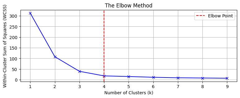
Fig. 1 Within-Cluster-Sum of Squares (WCSS) loss versus K

• Plot $K$ vs. inertia (WCSS)
• Look for an “elbow” where improvements slow down

2. Silhouette Score

• Measures separation vs. compactness:

\[s(i) = \frac{b(i) - a(i)}{\max(a(i), b(i))}\]

• Choose $K$ that maximizes average silhouette

3. Gap Statistic

• Compares clustering performance to random uniform data

\[\text{Gap}(K) = \mathbb{E}[\log(W_K^{\text{ref}})] - \log(W_K)\]

• Choose $K$ where gap is largest or flattens

4. Domain Knowledge

• Use task-specific or semantic insight to set $K$

---

📈 Summary Table

Method	Output	Pros	Cons
Random Init	Centroids	Fast	High collapse risk
k-means++	Centroids	Low collapse, better convergence	Slightly slower
Elbow	Optimal $K$	Simple, visual	Subjective
Silhouette	Optimal $K$	Captures quality of clustering	Expensive for large datasets
Gap Statistic	Optimal $K$	Strong theoretical foundation	Computationally heavy
Domain Knowledge	Optimal $K$	Expert-driven	May not always be available

---

🚀 Next Steps

• Use k-means++ for better initialization
• Choose $K$ via elbow + silhouette for practical datasets
• Combine PCA/t-SNE visualization with clustering to validate