Decision Tree Tutorial
Part 1: What Is a Decision Tree?
A Decision Tree is a recursive, rule-based model that partitions the feature space $\mathbb{R}^n$ into disjoint regions and assigns a prediction to each region. It works by splitting the dataset at each node based on feature values to reduce some measure of impurity or error.
Part 2: Splits and Split Criteria
A split is a binary partition of your dataset using a feature $x_j$ and a threshold $t$:
- Left Child: ${x \mid x_j \leq t}$
- Right Child: ${x \mid x_j > t}$
We want to pick the split that results in the most homogeneous child nodes (lowest impurity or error).
We use a greedy algorithm to find the best (feature, threshold) pair by minimizing:
$L_{\text{split}} = \frac{n_L}{n} L_L + \frac{n_R}{n} L_R$
Where:
- $L_L, L_R$: loss of the left and right child
- $n_L, n_R$: number of samples in left and right
- $n = n_L + n_R$
Part 3: Classification Losses
Gini Impurity:
\[G(S) = \sum_{c=1}^{C} p(c) (1 - p(c)) = 1 - \sum_{c=1}^{C} p(c)^2\]The Gini impurity measures how often a randomly chosen element from the set would be incorrectly labeled if it were randomly labeled according to the distribution of labels in the subset. Kind of the expected value of miss-classification.
The term $p(c)^2$ reflects the probability of correctly guessing the label if you sample twice with replacement:
- $p(c)^2$: probability that two independent samples from the node belong to class $c$.
- $\sum p(c)^2$: total probability of correct matches.
- So $1 - \sum p(c)^2$: total probability of mismatches → this is the impurity.
The square emphasizes that a node with one dominant class (large $p(c)$) gets much lower Gini, reinforcing purity.
Entropy:
\[H(S) = -\sum_{c=1}^{C} p(c) \log_2 p(c)\]Entropy comes from information theory. It measures the expected number of bits required to encode a label drawn at random.
- When all classes are equally likely → maximum entropy.
- When one class dominates → entropy is near zero.
By minimizing entropy after a split, we aim to move towards certainty (low disorder). This means the region is more “pure”, with fewer mixed-class samples.
How is $p(c)$ defined?
Given $n$ samples in a node and $n_c$ samples that belong to class $c$:
\[p(c) = \frac{n_c}{n}\]It represents the empirical probability of class $c$ in the current node. Since the total number of samples in the node is $n$, we have:
\[\sum_{c=1}^{C} p(c) = 1\]Part 4: Regression Loss
Mean Squared Error (MSE):
\[L(S) = \frac{1}{n} \sum_{i=1}^{n} (y_i - \bar{y})^2 = \text{Var}(S)\]- $y_i$ refers to the true target value of the $i^{th}$ training sample within the current node.
- $\bar{y}$ is the mean of all $y_i$ values in the node (i.e., the prediction the model will output for all samples in this region).
- So this formula measures how far each true value $y_i$ is from the average $\bar{y}$, and squares that distance to penalize larger deviations more.
This is the mean squared error (MSE), and it’s used to quantify how well a node’s prediction (the average) fits the actual values.
Part 5: Greedy Training Strategy
At each node:
- Loop through every feature.
-
For each unique threshold in that feature:
- Split the dataset.
- Compute child losses.
- Compute $L_{\text{split}}$.
- Choose the split with minimum total loss.
This is greedy: no backtracking or lookahead.
Depth-Based Splitting
Let the user specify a maximum depth $D$. Starting from the root (depth 0), recursively split both child nodes, regardless of which has higher or lower loss. That is:
- Even if one child has a worse loss than the other, both children are grown recursively to the next depth.
- The selection of the split is based on minimizing the total weighted loss of both children combined.
- This is a key property: you do not pick just one child to split. Once the best split is chosen, both the left and right child nodes become candidates for further recursive splitting (unless they hit a stopping condition like max depth or pure node).
This strategy allows the tree to grow into a full binary tree of depth $D$ (if data allows), where every node potentially splits into two children, recursively.
Pseudocode: Tree Growth with Depth Constraint
function grow_tree(dataset, depth):
    if stopping_condition_met(dataset, depth):
        return Leaf(value = compute_leaf_value(dataset))

    best_feature, best_threshold = find_best_split(dataset)
    left_subset, right_subset = split_dataset(dataset, best_feature, best_threshold)

    left_child = grow_tree(left_subset, depth + 1)
    right_child = grow_tree(right_subset, depth + 1)

    return Node(feature=best_feature, threshold=best_threshold, left=left_child, right=right_child)

function stopping_condition_met(dataset, depth):
    return (depth >= max_depth) or (all_same_class(dataset)) or (dataset too small)
This recursive algorithm ensures that once a split is selected, both child nodes are expanded independently — not just the better one.
Tree Representation and Inference
- Each node stores a feature and threshold.
- Each leaf stores a prediction (mean or majority class).
Inference in a Decision Tree
Once the tree is trained, inference is done by following a decision path from the root to a leaf node based on the input features.
Procedure:
- Start at the root node.
-
At each internal node:
- If the input feature value satisfies the condition (e.g., $x[j] \leq t$), move to the left child.
- Otherwise, move to the right child.
- Repeat this process recursively until a leaf node is reached.
-
The prediction is the value stored in the leaf:
- For classification: the majority class in the node.
- For regression: the mean target value of the node’s samples.
Leaf nodes in a tree are decision makers, so we traverse all the tree until we hit a leaf. Each leaf decides on part of the dataset.
Time Complexity: Inference is very fast — $\mathcal{O}(D)$, where $D$ is the depth of the tree, because only one path from root to leaf is followed.
This path-based traversal makes decision trees highly interpretable and efficient for real-time prediction tasks.
Part 6A: Classification Example
Dataset:
| Sample | Weight (g) | Class |
|---|---|---|
| A | 150 | 0 |
| B | 160 | 0 |
| C | 170 | 0 |
| D | 180 | 1 |
| E | 200 | 1 |
Depth 0: Root Node
Try split at threshold = 165:
- Left: $$150, 160] → Class = 0 → $G_L = 0$
- Right: \(170, 180, 200] → Classes =\)0, 1, 1] → $p(0) = \frac{1}{3}, p(1) = \frac{2}{3}$ → $G_R = \frac{4}{9}$
- Weighted Gini: $\frac{2}{5} \cdot 0 + \frac{3}{5} \cdot \frac{4}{9} = \frac{4}{15} \approx 0.266$
Depth 1:
Left child ($$150, 160]) → Pure → Leaf = 0
Right child ($$170, 180, 200])
-
Try threshold = 175:
- Left: $$170] → Class = 0 → $G = 0$
- Right: $$180, 200] → Class = 1 → $G = 0$
- Weighted Gini: $\frac{1}{3} \cdot 0 + \frac{2}{3} \cdot 0 = 0$
Perfect split → Both children are pure.
Final Tree Table:
| Depth | Node | Samples | Gini | Split | Left Child | Right Child |
|---|---|---|---|---|---|---|
| 0 | Root | A–E | 0.48 | Weight ≤ 165 | A, B | C, D, E |
| 1 | Left of root | A, B | 0 | — | Leaf: 0 | — |
| 1 | Right of root | C, D, E | 0.44 | Weight ≤ 175 | C (Leaf: 0) | D, E (Leaf: 1) |
Tree growth terminates as all leaves are pure or max depth is reached.
Part 6B: Regression Example
Dataset:
| Sample | Size | Price |
|---|---|---|
| A | 1100 | 200 |
| B | 1300 | 240 |
| C | 1500 | 270 |
| D | 1700 | 310 |
| E | 1900 | 350 |
Root Node (Depth 0):
- Try threshold: Size $\leq 1400$
- Left: A, B → Mean = 220 → MSE = $\frac{(200-220)^2 + (240-220)^2}{2} = 400$
- Right: C, D, E → Mean = 310 → MSE = $\frac{(270-310)^2 + (310-310)^2 + (350-310)^2}{3} = 533.33$
- Weighted MSE = $\frac{2}{5} \cdot 400 + \frac{3}{5} \cdot 533.33 = 480$
Depth 1:
- Left child is pure enough or has small data → stop
-
Right child: C, D, E
-
Try threshold: Size $\leq 1600$
- Left: C → Mean = 270, MSE = 0
- Right: D, E → Mean = 330, MSE = $\frac{(310-330)^2 + (350-330)^2}{2} = 400$
- Weighted MSE = $\frac{1}{3} \cdot 0 + \frac{2}{3} \cdot 400 = 266.67$
-
Final Tree Table:
| Depth | Node | Samples | Split | MSE | Prediction |
|---|---|---|---|---|---|
| 0 | Root | A–E | Size ≤ 1400 | 480 | |
| 1 | Left of Root | A, B | — | 400 | Mean = 220 |
| 1 | Right of Root | C, D, E | Size ≤ 1600 | 266.67 | |
| 2 | Left | C | — | 0 | Mean = 270 |
| 2 | Right | D, E | — | 400 | Mean = 330 |
Part 7: Tree Pruning
Decision trees can easily overfit the training data by creating very specific branches for rare patterns. To prevent this, we apply pruning, which simplifies the tree structure.
Why Prune?
- Reduce overfitting
- Improve generalization
- Shrink model size
Types of Pruning
-
Pre-pruning (early stopping)
-
This stops tree growth during training based on certain conditions:
- Max depth: Stop splitting further once the tree reaches a specified depth.
- Min samples per node: Only allow a split if a node has more than a certain number of samples.
- Min impurity decrease: Stop splitting if the reduction in impurity (e.g. Gini or entropy) is less than a small threshold.
-
Pre-pruning is fast and easy to implement, but can miss optimal splits that occur later in the tree.
-
-
Post-pruning (cost-complexity pruning)
- The tree is grown to full depth first (or nearly full).
- Then, starting from the leaves, we consider removing splits (i.e., replacing internal nodes with leaves).
- A split is removed if it does not significantly reduce error on a validation set.
- This process simplifies the tree while ensuring it still performs well.
Cost-Complexity Pruning (CCP)
Define an objective function:
\[R_\alpha(T) = R(T) + \alpha |T|\]- $R(T)$: empirical error (e.g. misclassification rate, Gini, entropy) of tree $T$
- $\mid T\mid$: number of terminal (leaf) nodes
- $\alpha$: regularization parameter controlling the trade-off between accuracy and simplicity
We prune the tree by selecting subtrees that minimize $R_\alpha(T)$. Larger $\alpha$ encourages simpler trees. CCP is used in many implementations such as scikit-learn’s DecisionTreeClassifier.
Decision trees can easily overfit the training data by creating very specific branches for rare patterns. To prevent this, we apply pruning, which simplifies the tree structure.
Part 8: Pros and Cons of Decision Trees
✅ Advantages:
- Interpretability: Easy to visualize and explain. You can follow a decision path.
- No data normalization needed: Trees are invariant to feature scaling.
- Handles mixed data types: Works with numerical and categorical features.
- Fast inference: Only one path is followed per prediction — $\mathcal{O}(D)$.
- Feature selection built-in: Trees automatically select informative features.
❌ Disadvantages:
- Overfitting: Deep trees often memorize the training data.
- Instability: Small changes in the data can lead to different trees (high variance).
- Bias towards features with more splits: Features with more values might dominate splits.
- Greedy decisions: Local optima are found; there’s no guarantee of global optimality.
- Hard to learn smooth functions: Unlike linear models or kernel methods.
Part 9: Summary Table
| Task | Loss Function | Leaf Output |
|---|---|---|
| Classification | Gini / Entropy | Majority class |
| Regression | MSE / Variance | Mean value |
Appendix
In a decision tree, each split decision compares a single feature against a threshold—not a multidimensional combination of features.
Key Concepts:
-
Univariate Splits (Most Common):
- At each internal node, the tree chooses one feature $f_j$ and finds the best threshold $t$ to split the data.
-
The decision rule is:
\[\text{If } x_j \leq t \text{ go left, else go right}\] - This means yes, there is one threshold per feature tested — but only one feature is tested per node.
-
How the feature and threshold are chosen:
- During training, for each node, the algorithm evaluates all features $j \in {1, \ldots, m}$ and for each feature considers all possible thresholds $t$.
- For each (feature, threshold) pair, it computes a split score using criteria like Gini impurity, entropy, or variance reduction.
- The (feature, threshold) pair with the best score is chosen to split the data.
-
Multivariate Splits (Rare):
- These use linear combinations like $\mathbf{w}^T \mathbf{x} \leq t$, where multiple features are involved.
- This is not standard in classical decision trees, but exists in some variants like oblique decision trees.
- These are computationally more complex and less interpretable.
Two Feature Decision Tre Example
Here is a compact worked example, two numerical features, three classes, Gini impurity, greedy CART splits.
Dataset, eight points
| id | size | weight | class |
|---|---|---|---|
| 1 | 1 | 1 | A |
| 2 | 2 | 1 | A |
| 3 | 2 | 2 | B |
| 4 | 3 | 1 | A |
| 5 | 3 | 3 | B |
| 6 | 4 | 3 | C |
| 7 | 5 | 4 | C |
| 8 | 5 | 2 | B |
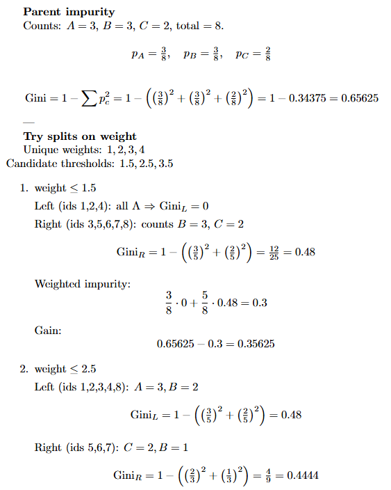
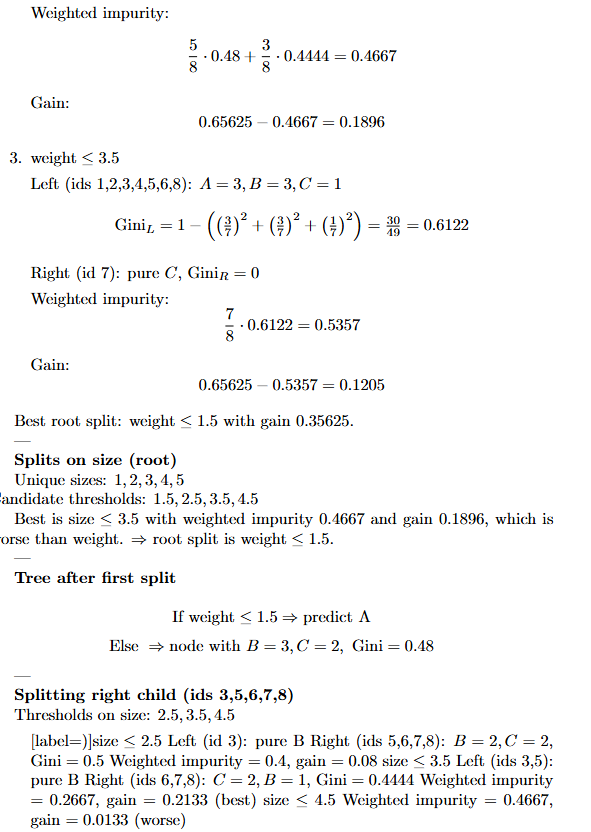
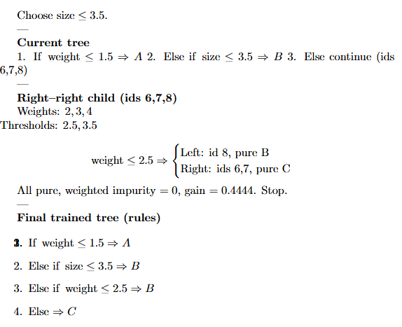
This example shows exactly how you compute candidate thresholds, child impurities, weighted impurities, and information gain at each step, until either purity is reached or stopping rules say to create a leaf.
Core Algorithm
Core idea of how a standard decision tree is trained:
At each node during training:
- Take the subset of data that reaches this node.
-
For every feature (or a random subset if you are training a random forest):
- Try possible split points (thresholds for numerical features, category partitions for categorical features).
- Compute the impurity reduction (information gain, Gini reduction, variance reduction, etc.).
- Pick the feature and split point with the largest impurity reduction. That feature is used at this node, and the data is divided accordingly.
- Repeat the process separately for the left and right subsets (recursion).
So we don’t pre-decide an order of features. At each node, the tree re-evaluates all candidate features again and “switches” to whichever one is most useful at that point in the data.
Summary:
- ✅ Standard decision trees use one feature and one threshold per node.
- ❌ They do not compare multidimensional feature combinations by default.
- ✅ Each feature considered has its own candidate thresholds during training.
- 🧠 Extensions exist (e.g., oblique trees) for multivariate splits, but they are not part of classic decision trees like CART or ID3.