Understanding DETR: Object Detection with Transformers
Good video Here
Table of Contents
- Introduction
- Why Transformers for Object Detection?
- DETR Architecture Overview
- Encoder Detailed Explanation
- Decoder Detailed Explanation
- Remarks on the Tensor Size, and Architecture Wrap up
- Remarks on the Positional Embedding
- Loss Functions and Bipartite Matching
- Conclusion
Introduction
The Detection Transformer (DETR) is a novel approach to object detection that leverages Transformers, which were originally designed for sequence-to-sequence tasks like machine translation. Introduced by Carion et al. in 2020, DETR simplifies the object detection pipeline by eliminating the need for hand-crafted components like anchor generation and non-maximum suppression (NMS).
Why Transformers for Object Detection?
Traditional object detection models rely on convolutional neural networks (CNNs) with added complexities like region proposal networks, anchor boxes, and NMS. Transformers offer a simpler and more unified architecture by modeling object detection as a direct set prediction problem.
Reasons for Using Transformers:
- Global Context Modeling: Transformers can capture long-range dependencies, making them suitable for understanding global context in images.
- Simplified Pipeline: Eliminates the need for NMS and anchor boxes, reducing hyperparameters.
- Set Prediction: Treats object detection as a set prediction problem, which aligns well with the permutation-invariant nature of Transformers.
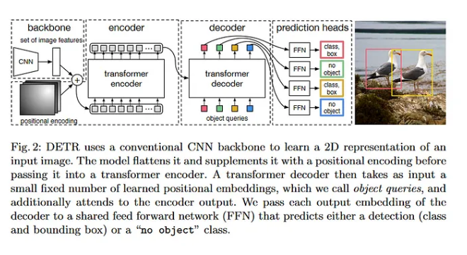
DETR Architecture Overview
DETR consists of three main components:
- Backbone CNN: Extracts feature maps from the input image.
- Transformer Encoder: Processes the feature maps to capture global context.
- Transformer Decoder: Generates object predictions using learned object queries.
Below is a high-level diagram of the DETR architecture:
Input Image --> Backbone CNN --> Transformer Encoder --> Transformer Decoder --> Predictions
Encoder Detailed Explanation
Role of the Encoder
The encoder processes the feature map from the backbone and outputs a sequence of context-rich feature representations. It models the relationships between all positions in the feature map, capturing global information.
Below is a detailed, step-by-step breakdown of the DETR encoder. The DETR encoder is essentially a stack of standard Transformer encoder layers, each composed of:
- Self-Attention (attention over the input sequence itself)
- Feed-Forward Network (FFN)
We will detail the mathematical operations, their dimensions, and provide a PyTorch-like pseudo-code snippet with inline comments. We will assume the following for simplicity:
- Model dimension: \(D\) (e.g., 256)
- Number of heads: \(H\) (e.g., 8)
- Per-head dimension: \(d_{head} = D/H\) (e.g., 256/8 = 32)
- Number of encoder tokens: \(N_{enc} = H' \times W'\), where \(H'\) and \(W'\) are spatial dims of the feature map after the backbone and projection (for instance, \(N_{enc} = 2000\)).
- Batch size: \(B\) (e.g., 2 or 4, etc.)
- Number of encoder layers: \(L\) (e.g., 6)
Input to the Encoder:
-
The DETR encoder receives as input a 2D feature map from a CNN backbone, flattened into a sequence of feature vectors. After positional encoding and a linear projection:
\[\text{enc}_\text{inp} \in \mathbb{R}^{B \times N_{enc} \times D}\]Each element is a \(D\)-dim vector representing a specific spatial location in the feature map.
Encoder Layer Workflow:
Each encoder layer consists of:
- Self-Attention: The encoder attends to itself. Each token in the input sequence attends to all others (including itself).
- Feed-Forward Network: A two-layer MLP applied to each token independently.
Mathematical Formulation:
Let \(\mathbf{X}^{(l)}\) be the input to the \(l\)-th encoder layer. Initially, \(\mathbf{X}^{(0)} = \text{enc}_\text{inp}\).
- The input layer adds positional embedding to \(\mathbf{X}^{(0)}\) therefore we have
-
Multi-Head Self-Attention:
Compute queries, keys, and values from \(\mathbf{X}^{(l)}\):
\[Q = \mathbf{X}^{(l)}W_Q, \quad K = \mathbf{X}^{(l)}W_K, \quad V = \mathbf{X}^{(l)}W_V\]Dimensions:
- \(\mathbf{X}^{(l)}, Q, K, V \in \mathbb{R}^{B \times N_{enc} \times D}\).
Reshape for multi-heads:
\(Q' = \text{reshape}(Q, [B, N_{enc}, H, d_{head}]) \rightarrow \mathbb{R}^{B \times H \times N_{enc} \times d_{head}}\) Similarly for \(K', V'\).
Compute attention scores:
\[A = \text{softmax}\left(\frac{Q'K'^{T}}{\sqrt{d_{head}}}\right) \in \mathbb{R}^{B \times H \times N_{enc} \times N_{enc}}\]Apply attention to values:
\[O' = A V' \in \mathbb{R}^{B \times H \times N_{enc} \times d_{head}}\]Reshape back:
\[O = \text{reshape}(O', [B, N_{enc}, D])W_{O}\]Residual + LayerNorm:
\[\mathbf{X}^{(l)} := \text{LayerNorm}(\mathbf{X}^{(l)} + O)\] -
Feed-Forward Network (FFN):
The FFN is typically two linear layers with a ReLU in between:
\[\mathbf{X}^{(l)} := \mathbf{X}^{(l)} + \text{Dropout}( \text{ReLU}(\mathbf{X}^{(l)}W_1 + b_1)W_2 + b_2 )\]Then another LayerNorm:
\[\mathbf{X}^{(l)} := \text{LayerNorm}(\mathbf{X}^{(l)})\]
After \(L\) encoder layers, the output \(\mathbf{X}^{(L)}\) is used by the decoder as “memory”.
Pseudo-Code in PyTorch-Like Style
import torch
import torch.nn as nn
import torch.nn.functional as F

class TransformerEncoderLayer(nn.Module):
    def __init__(self, d_model=256, nhead=8, dim_feedforward=2048, dropout=0.1):
        super().__init__()

        # Multi-head self-attention
        self.self_attn = nn.MultiheadAttention(embed_dim=d_model, num_heads=nhead, dropout=dropout)

        # Feed-forward network
        self.linear1 = nn.Linear(d_model, dim_feedforward)
        self.linear2 = nn.Linear(dim_feedforward, d_model)

        self.norm1 = nn.LayerNorm(d_model)
        self.norm2 = nn.LayerNorm(d_model)

        self.dropout1 = nn.Dropout(dropout)
        self.dropout2 = nn.Dropout(dropout)

    def forward(self, src):
        # src: (B, N_enc, D)

        # PyTorch's MultiheadAttention expects (N_enc, B, D)
        src_transposed = src.transpose(0, 1)  # (N_enc, B, D)

        # Self-attention
        # Query=Key=Value=src itself
        attn_output, _ = self.self_attn(src_transposed, src_transposed, src_transposed)
        # attn_output: (N_enc, B, D)

        # Residual + LayerNorm
        src = src + self.dropout1(attn_output.transpose(0, 1))  # back to (B, N_enc, D)
        src = self.norm1(src)  # (B, N_enc, D)

        # Feed-Forward Network
        ff_output = self.linear2(F.relu(self.linear1(src)))  # (B, N_enc, D)

        # Residual + LayerNorm
        src = src + self.dropout2(ff_output)
        src = self.norm2(src)  # (B, N_enc, D)

        return src


# Example usage:
B = 2
N_enc = 2000
D = 256

enc_input = torch.randn(B, N_enc, D)  # (B, N_enc, D)

encoder_layer = TransformerEncoderLayer(d_model=D, nhead=8, dim_feedforward=2048)

# Pass through one encoder layer
out = encoder_layer(enc_input)
# out: (B, N_enc, D)
Inline Comments and Dimensions:
enc_input: Shape(B, N_enc, D). The flattened feature map with positional encodings added.- Internally, before passing to
nn.MultiheadAttention, we transpose to(N_enc, B, D)because PyTorch’s multi-head attention layer expects(sequence_length, batch_size, embed_dim)format.
Multi-head Self-Attention Step-by-Step:
src_transposed:(N_enc, B, D)- Attention is computed across
N_enctokens. attn_output:(N_enc, B, D)
After attention, we transpose back to (B, N_enc, D) and apply residual + LayerNorm.
Feed-Forward Network:
- Apply linear layers:
(B, N_enc, D) -> (B, N_enc, dim_feedforward) -> ReLU -> (B, N_enc, D) - Residual + LayerNorm.
You stack L such layers to form the full encoder. The final encoder output is (B, N_enc, D) and is fed into the DETR decoder as the “memory”.
Summary of Encoder:
This provides a detailed workflow of a single DETR encoder layer:
- Receives a batch of sequences
(B, N_enc, D). - Applies multi-head self-attention over the sequence.
- Applies a feed-forward network to each token independently.
- Each sub-layer is followed by residual connection and LayerNorm.
-
After
Llayers, we get the final encoder output that represents the transformed image features. Input Shapes to the Decoder: -
Encoder Output: \(\text{enc}_\text{out} \in \mathbb{R}^{B \times N_{enc} \times D}\)
This is the output from the Transformer encoder. It represents a set of \(N_{enc}\) feature vectors, each of dimension \(D\). - Query Embeddings: \(\text{queries} \in \mathbb{R}^{B \times N_{query} \times D}\)
These are learned positional embeddings (object queries) that serve as the initial input to the decoder. Initially, at the first decoder layer, these queries are usually a set of learned parameters (not dependent on the image content). For subsequent layers, they are the output of the previous decoder layer.
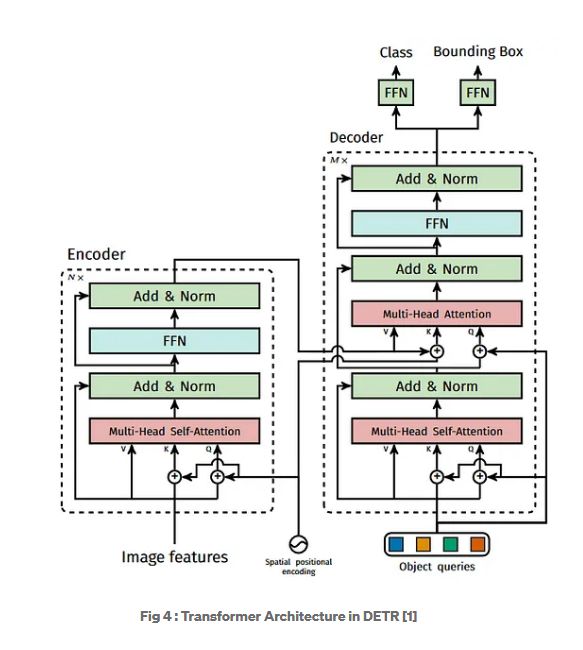
Decoder Layer Workflow:
A single decoder layer takes queries and the encoder output and does:
- Self-Attention (on queries):
- Compute \(Q, K, V\) for self-attention from the current queries.
- Perform multi-head attention.
- Add & normalize (residual connection + LayerNorm).
- Cross-Attention (queries attend to encoder output):
- Compute \(Q\) from queries, \(K, V\) from encoder output.
- Perform multi-head cross-attention.
- Add & normalize (residual connection + LayerNorm).
- Feed-Forward Network (FFN):
- A two-layer MLP (linear -> ReLU -> linear).
- Add & normalize (residual connection + LayerNorm).
The output of the last decoder layer is used to produce object class predictions and bounding box predictions.
Mathematical Formulation
Self-Attention:
For each decoder layer, given the current query embeddings \(\mathbf{Q}^{(l)}\):
-
Project to queries, keys, and values for self-attention:
\[Q = \mathbf{Q}^{(l)}W_{Q}^{self}, \quad K = \mathbf{Q}^{(l)}W_{K}^{self}, \quad V = \mathbf{Q}^{(l)}W_{V}^{self}\]Dimensions:
- \[Q, K, V \in \mathbb{R}^{B \times N_{query} \times D}\]
-
Reshape for multi-heads:
\[Q' = \text{reshape}(Q, [B, N_{query}, H, d_{head}]) \rightarrow \mathbb{R}^{B \times H \times N_{query} \times d_{head}}\]Similarly for \(K', V'\).
-
Compute attention weights:
\[A = \text{softmax}\left(\frac{Q'K'^{T}}{\sqrt{d_{head}}}\right) \in \mathbb{R}^{B \times H \times N_{query} \times N_{query}}\] -
Weighted sum:
\[O' = A V' \in \mathbb{R}^{B \times H \times N_{query} \times d_{head}}\] -
Reshape and project back:
\[O = \text{reshape}(O', [B, N_{query}, D])W_{O}^{self}\] -
Residual + LayerNorm:
\[\mathbf{Q}^{(l)} := \text{LayerNorm}(\mathbf{Q}^{(l)} + O)\]
Cross-Attention:
Now using the updated queries \(\mathbf{Q}^{(l)}\):
-
Project queries, keys, values for cross-attention:
\[Q = \mathbf{Q}^{(l)} W_{Q}^{cross}, \quad K = \text{enc}_\text{out}W_{K}^{cross}, \quad V = \text{enc}_\text{out}W_{V}^{cross}\]Dimensions:
- \[Q \in \mathbb{R}^{B \times N_{query} \times D}\]
- \[K, V \in \mathbb{R}^{B \times N_{enc} \times D}\]
-
Reshape for multi-heads and compute attention similarly:
\[A = \text{softmax}\left(\frac{Q'K'^{T}}{\sqrt{d_{head}}}\right) \in \mathbb{R}^{B \times H \times N_{query} \times N_{enc}}\]Here \(Q' \in \mathbb{R}^{B \times H \times N_{query} \times d_{head}}\)
and \(K' \in \mathbb{R}^{B \times H \times N_{enc} \times d_{head}}\). -
Compute:
\[O' = A V' \in \mathbb{R}^{B \times H \times N_{query} \times d_{head}}\]Reshape and project back to \(D\):
\[O = \text{reshape}(O', [B, N_{query}, D])W_{O}^{cross}\] -
Residual + LayerNorm:
\[\mathbf{Q}^{(l)} := \text{LayerNorm}(\mathbf{Q}^{(l)} + O)\]
Feed-Forward Network:
-
Two-layer MLP:
\[\mathbf{Q}^{(l)} := \mathbf{Q}^{(l)} + \text{Dropout}(\text{ReLU}(\mathbf{Q}^{(l)}W_1 + b_1)W_2 + b_2)\] -
LayerNorm again:
\[\mathbf{Q}^{(l)} := \text{LayerNorm}(\mathbf{Q}^{(l)})\]
This completes one decoder layer. The decoder stacks \(L\) such layers.
Pseudo-Code in PyTorch-Like Style
import torch
import torch.nn as nn
import torch.nn.functional as F

class TransformerDecoderLayer(nn.Module):
    def __init__(self, d_model=256, nhead=8, dim_feedforward=2048, dropout=0.1):
        super().__init__()

        # Multi-head attention layers
        self.self_attn = nn.MultiheadAttention(embed_dim=d_model, num_heads=nhead, dropout=dropout)
        self.cross_attn = nn.MultiheadAttention(embed_dim=d_model, num_heads=nhead, dropout=dropout)

        # Feed-forward network
        self.linear1 = nn.Linear(d_model, dim_feedforward)
        self.linear2 = nn.Linear(dim_feedforward, d_model)

        self.norm1 = nn.LayerNorm(d_model)
        self.norm2 = nn.LayerNorm(d_model)
        self.norm3 = nn.LayerNorm(d_model)

        self.dropout1 = nn.Dropout(dropout)
        self.dropout2 = nn.Dropout(dropout)
        self.dropout3 = nn.Dropout(dropout)

    def forward(self,
                tgt,        # (B, N_query, D) queries to be decoded
                memory):    # (B, N_enc, D) from encoder
        # Self-attention block
        # tgt: (B, N_query, D)
        # we need to transpose to (N_query, B, D) for nn.MultiheadAttention
        q = k = tgt.transpose(0, 1)  # (N_query, B, D)
        v = q
        tgt2, _ = self.self_attn(q, k, v)  # attn over queries themselves
        # tgt2: (N_query, B, D)
        tgt = tgt + self.dropout1(tgt2)  # residual
        tgt = self.norm1(tgt)  # (N_query, B, D)

        # Cross-attention block
        # Query: tgt, Key+Value: memory
        # memory: (B, N_enc, D) -> (N_enc, B, D)
        q = tgt
        k = memory.transpose(0, 1)    # (N_enc, B, D)
        v = memory.transpose(0, 1)    # (N_enc, B, D)
        tgt2, _ = self.cross_attn(q, k, v)
        tgt = tgt + self.dropout2(tgt2)
        tgt = self.norm2(tgt)  # (N_query, B, D)

        # Feed-Forward Network
        # tgt: (N_query, B, D)
        tgt2 = self.linear2(F.relu(self.linear1(tgt)))
        tgt = tgt + self.dropout3(tgt2)
        tgt = self.norm3(tgt)  # (N_query, B, D)

        # return (B, N_query, D)
        return tgt.transpose(0, 1)

# Example usage:
B = 2
N_query = 100
N_enc = 2000
D = 256

queries = torch.randn(B, N_query, D)     # (B, N_query, D)
enc_out = torch.randn(B, N_enc, D)       # (B, N_enc, D)

decoder_layer = TransformerDecoderLayer(d_model=D, nhead=8, dim_feedforward=2048)

# Pass through one decoder layer
out = decoder_layer(queries, enc_out)
# out: (B, N_query, D)
Inline Comments and Dimensions:
queries: Shape(B, N_query, D). The queries for objects we want to detect.enc_out: Shape(B, N_enc, D). The memory from the encoder (flattened image features).
In the forward call of TransformerDecoderLayer:
- First self-attention:
- Input:
tgtof shape(B, N_query, D). nn.MultiheadAttentionexpects(N_query, B, D), so we transpose: now(N_query, B, D).- Self-attention keys/values are the same queries.
- Output
tgt2:(N_query, B, D). - Residual + LayerNorm: still
(N_query, B, D).
- Input:
- Cross-attention:
q = tgt:(N_query, B, D)k, v = memory.transpose(0,1):(N_enc, B, D)- Output
tgt2:(N_query, B, D) - Residual + LayerNorm:
(N_query, B, D)
- FFN:
- Two linear layers:
(N_query, B, D) -> (N_query, B, dim_feedforward) -> ReLU -> (N_query, B, D) - Residual + LayerNorm:
(N_query, B, D)
- Two linear layers:
- Finally, transpose back to
(B, N_query, D).
Remarks on the Tensor Size, and Architecture Wrap Up:
- The cross-attention in the DETR decoder is computed between a set of N_query(here N_query = M) queries and N_enc (here N_enc = N) encoder output tokens. Therefore, the cross-attention weight matrix has dimensions (N_query × N_enc).
- The encoder outputs a sequence of shape (N_enc, D), where N_enc is typically the flattened spatial dimension of the image features and D is the model dimension.
- The decoder queries consist of N_query learned embeddings, each of dimension D.
- For cross-attention, the query (Q) matrix is of shape (N_query, D), and the key (K) and value (V) matrices derived from the encoder output are of shape (N_enc, D).
Detailed Explanation:
- Encoder Output Size:
DETR first processes an input image through a backbone CNN (e.g., ResNet-50), resulting in a feature map of size(C, H', W'). These features are then flattened and projected into aD-dimensional space. Let’s define:H'andW'are the spatial dimensions of the downsampled feature map after the backbone and possibly additional projections.- The total number of spatial positions is
N_enc = H' * W'. - Each position is represented by a
D-dimensional vector after linear projection.
Thus, after positional encoding and passing through the Transformer encoder (with multiple layers), the encoder output is a sequence of shape:
\[\text{Encoder Output} \in \mathbb{R}^{N_{\text{enc}} \times D}, \quad \text{where } N_{\text{enc}} = H'W'\] -
Decoder Queries:
\[\text{Decoder Queries} \in \mathbb{R}^{N_{\text{query}} \times D}, \quad \text{where } N_{\text{query}} \text{ is often set to 100}\]
The DETR decoder uses a fixed set of N_query learned object queries. Each query is aD-dimensional embedding. These queries are independent of the input image content; they are trained to attend to different parts of the encoder output to detect objects. So the query set is:Each decoder layer uses these queries to attend to the encoder outputs and produce refined queries (representations) that eventually lead to object predictions.
- Cross-Attention in the Decoder:
In a standard Transformer cross-attention module, you have three key matrices: Q (query), K (key), and V (value). For cross-attention in the DETR decoder:
- Q (Query): Derived from the decoder queries. After a linear projection, these will still have dimension
(N_query, D). - K (Key) and V (Value): Derived from the encoder output. After linear projections, these remain
(N_enc, D).
Concretely:
-
Q is obtained by applying a linear transformation to the decoder queries:
\[Q \in \mathbb{R}^{N_{\text{query}} \times D}\] -
K and V are obtained by applying linear transformations to the encoder output:
\[K \in \mathbb{R}^{N_{\text{enc}} \times D}, \quad V \in \mathbb{R}^{N_{\text{enc}} \times D}\]
- Q (Query): Derived from the decoder queries. After a linear projection, these will still have dimension
-
Cross-Attention Computation: The attention weights are computed as:
\[\text{Attention} = \text{softmax}\left(\frac{QK^T}{\sqrt{D}}\right) V\]Here,
QK^Tresults in a(N_query, N_enc)matrix:Qhas shape(N_query, D).K^Thas shape(D, N_enc).
Multiplying
\[QK^T \in \mathbb{R}^{N_{\text{query}} \times N_{\text{enc}}}\]Q (N_query, D)byK^T (D, N_enc)gives:This is the cross-attention weight matrix, which, after the softmax operation, is used to combine the values:
\[\text{Attention Output} = \text{softmax}(QK^T) V \in \mathbb{R}^{N_{\text{query}} \times D}\]
Summary of Dimensions:
- Encoder output:
(N_enc, D)whereN_enc = H' * W'. - Decoder queries:
(N_query, D)(e.g.,N_query = 100). - Cross-attention Q:
(N_query, D) - Cross-attention K and V:
(N_enc, D) - Cross-attention matrix (QK^T):
(N_query, N_enc)
This is the general scheme for the DETR architecture’s cross-attention dimensions.
Remarks on the Positional Embedding
Positional embeddings are re-applied to the keys during the decoder’s cross-attention to ensure that positional information is explicitly available when computing attention weights. Only the keys (and queries) get positional embeddings because the attention mechanism relies on the Q–K interaction to determine “where” to attend. Adding positional information to the values is not necessary for establishing spatial correspondence, and could distort the content features.
Detailed Explanation:
-
Positional Embeddings in Transformer Attention: In a Transformer, attention weights are computed using the queries (Q) and keys (K):
\[A = \text{softmax}\left( \frac{QK^T}{\sqrt{d_{head}}} \right).\]The values (V) are then aggregated using these attention weights. Thus, the determination of “where to attend” comes from the similarity of Q and K. By encoding positional information into K (and Q), the model can factor spatial position directly into the attention score calculation.
- Why Add Positional Embeddings Again to Keys in the Decoder?
- Encoder Output Already Contains Positional Information, Right?
The encoder output (“memory”) is influenced by the positional embeddings that were added at the encoder input stage. After passing through multiple self-attention layers, the encoder’s output features do carry implicit positional structure. However, the positional information is no longer explicitly represented as a simple additive signal. It’s been “distributed” throughout the representations by self-attention mixing.
- Encoder Output Already Contains Positional Information, Right?
- Queries in the Decoder Represent Object Queries (Learnable Embeddings)
The queries in DETR’s transformer decoder are object queries, which are learnable embeddings initialized randomly and updated during training. These queries do not correspond to specific spatial locations in the image but rather act as high-level object “slots” that extract information about different objects. Since these queries are not tied to spatial positions, there is no need to add positional embeddings. Keys (from Encoder) Represent Spatial Information
The keys and values in the decoder come from the encoder, which processes image features extracted from a CNN backbone. These feature maps retain spatial information about objects, so it is crucial to add positional encodings to the encoder’s outputs (keys) to provide spatial awareness. Without positional embeddings, the self-attention mechanism in the decoder would treat all key features as position-agnostic, making it harder to distinguish objects at different locations. Attention Mechanism in the Decoder
In the decoder, each query attends to all spatial positions (keys) in the encoded image features. Since the queries are not tied to specific locations, the positional information should only come from the keys to ensure the decoder can correctly localize objects.
In the decoder’s cross-attention, we explicitly add positional embeddings again to the keys. This ensures the positional cues are directly and cleanly available at the point of computing attention weights. The decoder’s cross-attention mechanism can then straightforwardly use these embeddings to differentiate locations. This step reinforces positional cues so that the decoder’s object queries (queries Q) can latch onto spatial locations (keys K) more easily and accurately.
-
Why Not Add Positional Embeddings to Values? The attention step involves:
\[\text{Attention}(Q,K,V) = \text{softmax}\left(\frac{QK^T}{\sqrt{d_{head}}}\right) V.\]-
Position is About “Where,” Not “What”:
The queries and keys are responsible for determining the attention weights — in other words, “where” to focus. Positional information guides this “where” by helping the model pick out relevant spatial locations. Thus, including positional embeddings in Q and K is sufficient to influence the attention weights spatially. -
Values Represent Content Features:
The values (V) contain the “what” information — the semantic content of each position. If we add positional embeddings to V, we’d be mixing positional signals into the final aggregated representation. This might unnecessarily entangle positional information with the actual content features. The model already knows where to attend from Q and K; once the location is selected, we just need to retrieve the raw content from V. Keeping V free of additional positional signals prevents overwriting or distorting the semantic information.
-
-
Design Choice Backed by Practice: This approach (adding positional embeddings to Q and K but not V) is a standard design in many Transformer variants. Position is crucial for attention weight calculation, but not necessary for the value aggregation step. This ensures a clean separation: Q and K handle “where,” while V focuses on “what.”
Summary:
- Re-applying positional embeddings to the keys in the decoder’s cross-attention explicitly reintroduces clear positional cues during the attention step, ensuring robust spatial reasoning.
- Positional embeddings are not added to values because it’s unnecessary for determining “where” to attend and could dilute the content information.
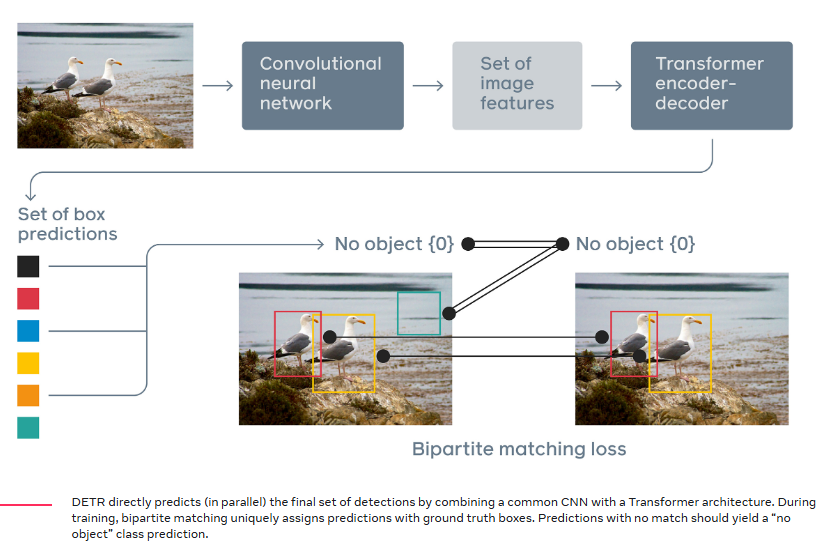
Loss Functions and Bipartite Matching
Overview:
DETR’s loss function and training procedure differ from traditional object detectors because it treats object detection as a direct set prediction problem. This approach removes the need for non-maximum suppression (NMS) and anchor generation. Instead, DETR predicts a fixed-size set of object “queries” and then finds a one-to-one matching between these predictions and the ground truth objects using the Hungarian algorithm. The loss is then computed based on this optimal matching.
Key Steps in DETR’s Loss Computation:
- Fixed-Size Predictions:
DETR outputs a fixed number of predictions (for example, 100 predictions per image). Each prediction consists of:
- A class probability distribution (including the “no object” or background class).
- A predicted bounding box (parameterized by its center coordinates, width, and height, or sometimes normalized coordinates).
Let’s denote:
- The set of predictions as \(\{\hat{y}_i\}_{i=1}^{N}\), where \(N\) is a fixed number like 100.
- Each \(\hat{y}_i\) includes \(\hat{p}_i(c)\) for each class \(c\) and a predicted bounding box \(\hat{b}_i\).
- Constituting Ground Truth:
The ground truth for an image typically consists of:
- A set of \(M\) ground truth objects \(\{y_j\}_{j=1}^{M}\) where each \(y_j\) includes a ground-truth class label \(c_j\) and a ground-truth bounding box \(b_j\).
DETR assumes \(M \leq N\). If there are fewer ground-truth objects than the number of predictions, the unmatched predictions should ideally represent the “no object” class.
-
Optimal Bipartite Matching with the Hungarian Algorithm: One critical innovation in DETR is how it determines which predicted query corresponds to which ground truth object. This is done via a one-to-one matching using the Hungarian (a.k.a. Kuhn-Munkres) algorithm.
Forming the Cost Matrix:
- First, DETR computes a cost for matching each predicted box \(\hat{y}_i\) with each ground truth object \(y_j\).
- The cost includes both classification and localization terms:
-
Classification Cost: This is typically the negative log-likelihood of the ground truth class under the predicted class distribution:
\[C_{\text{class}}(y_j, \hat{y}_i) = -\log \hat{p}_i(c_j)\] -
Bounding Box Localization Cost:
DETR uses a combination of:- L1 loss on bounding box coordinates: \(\| b_j - \hat{b}_i \|_1\)
-
Generalized IoU (GIoU) loss on bounding boxes:
\[C_{\text{box}}(y_j, \hat{y}_i) = \lambda_{\text{L1}}\| b_j - \hat{b}_i \|_1 + \lambda_{\text{GIoU}}(1 - \text{GIoU}(b_j, \hat{b}_i))\]
-
Thus, the total cost for matching ground-truth object \(j\) and predicted object \(i\) could be:
\[C(y_j, \hat{y}_i) = C_{\text{class}}(y_j, \hat{y}_i) + C_{\text{box}}(y_j, \hat{y}_i)\]Hungarian Matching:
- After forming the \(M \times N\) cost matrix (with \(M \leq N\)), the Hungarian algorithm is applied to find the global one-to-one matching between predictions and ground truth that yields the minimal total cost.
- This results in a permutation \(\sigma\) of \(\{1,\ldots,N\}\) (or a partial mapping if \(N>M\)) such that \(\sigma(j)\) is the index of the prediction matched to the ground-truth object \(j\).
-
Computing the Loss After Matching: Once the optimal matching is established, the loss is computed by summing over the matched pairs and also taking into account the unmatched predictions:
Matched Predictions: For each matched pair \((j, \sigma(j))\):
- Classification Loss: A cross-entropy loss for the matched prediction’s class distribution against the ground truth class. This encourages the matched prediction to classify correctly.
- Box Regression Loss: A combination of L1 loss and GIoU loss between the matched predicted box and the ground truth box.
Unmatched Predictions: For the predictions that are not matched to any ground truth object, the model expects them to predict the “no object” (or background) class. Thus, those predictions incur a classification loss pushing them towards predicting “no object.”
Formally, the final loss \(\mathcal{L}\) is:
\[\mathcal{L} = \sum_{j=1}^{M} [\mathcal{L}_{\text{class}}(y_j, \hat{y}_{\sigma(j)}) + \lambda_{\text{box}}\mathcal{L}_{\text{box}}(y_j, \hat{y}_{\sigma(j)})] + \sum_{i \notin \{\sigma(1), \ldots, \sigma(M)\}} \mathcal{L}_{\text{class}_\text{noobj}}(\hat{y}_{i})\]Where:
- \(\mathcal{L}_{\text{class}}\) is the cross-entropy loss for the correct class.
- \(\mathcal{L}_{\text{box}}\) includes both L1 and GIoU losses.
- \(\mathcal{L}_{\text{class}_\text{noobj}}\) is the loss that encourages predictions that aren’t matched to a real object to predict the “no object” class.
Summary:
- Ground Truth Constitution: The ground truth is simply the set of annotated bounding boxes and their classes for each image.
- Matching: DETR uses the Hungarian algorithm to find a unique, one-to-one assignment between the predicted set of objects (queries) and the ground-truth objects.
- Loss Function:
- A combined classification and box regression loss is computed only for matched predictions.
- Unmatched predictions are penalized if they fail to predict the “no object” class.
- The Hungarian matching ensures a fair and stable assignment, enabling an end-to-end set prediction that does not require post-processing like NMS.
Conclusion
DETR revolutionizes object detection by framing it as a direct set prediction problem using Transformers. The architecture simplifies the detection pipeline, removes the need for heuristic components like NMS, and provides a unified end-to-end trainable model.
Key Takeaways:
- Transformer Encoder: Captures global context in images.
- Transformer Decoder: Uses object queries to predict objects in parallel.
- Set-Based Loss with Bipartite Matching: Ensures unique assignment of predictions to ground truth objects.
By leveraging the strengths of Transformers, DETR opens new avenues for research and applications in object detection and beyond.
Panoptic Segmentation
for a better understanding of the actual science behind the segmentation head please look at this awesome Video